In our previous article, What Is Julia, and Why It Matters?, we discussed why Julia is so relevant today and made some comparisons between other similar languages, such as Python and R. We also mentioned some of its main characteristics and features, and concluded with some next steps to get started programming on Julia.
In this Blog Article, we’ll install Julia and an awesome VS Code extension that will make programming easier for us. We’ll also take a look at two notebook environments: Pluto.jl, a great Julia-specific notebook environment, and JupyterLab. We’ll set up an environment, install some packages, and cover several practical examples, where we will perform a general overview of Julia’s main functionalities. We will close this segment by recommending how to use Julia and some helpful next steps for those interested in this exciting, bleeding-edge programming language.
We’ll be using Julia scripts and reactive notebooks, which can be found in the Blog Article Repo. Datasets can also be found in the datasets repo folder.
What to expect
Although Julia is a relatively new language and doesn’t enjoy the vast IDE support that Python has (yet), we have limited options, but the ones currently available are superb and well-maintained. This segment will heavily rely on VS Code since it’s the IDE presently getting the most support. Some time ago, Juno was also well maintained, but efforts have now been transferred entirely to the VS Code extension. We will also use an extremely fun Julia-specific notebook environment called Pluto.jl, as well as the well-known JupyterLab. We will be using Microsoft Windows, but a similar installation process applies to other platforms, such as macOS & Linux. The rest of the article can be easily translated for other platforms.
Also, we’ll assume there is at least some knowledge or background in some programming language since Julia, despite being syntactically simple, can get complex quickly; Python should do just fine since they’re very similar syntaxis-wise.
We will not rigorously explore all of Julia’s functionalities since there is too much to cover. Instead, we will review a comprehensive set of hands-on examples to start programming in Julia from scratch.
Installation
For this segment, we will need to install four main components:
- The Julia programming language.
- Visual Studio Code.
- The Visual Studio Code Julia extension.
- The JuliaMono typeface.
We will also install some packages, which will come handy later on when we get to the pkg package manager.
1. Julia
We will first install the latest stable release of the Julia programming language. We can head to the official Julia Lang website downloads page. We will select the Windows 64-bit (installer). Once we have it, we’ll run the executable and follow the shown steps.
Adding Julia to PATH is important since this will ensure we can start the Julia REPL directly from our terminal without specifying the whole absolute path for the executable. This will be useful when creating our project environment and installing some packages.
If we missed this step for some reason, that’s perfectly fine. We can simply follow the steps below:
- Open Windows Run by using Windows Key + R.
- Type
rundll32 sysdm.cpl,EditEnvironmentVariablesand hit Enter. - Head to user variables.
- Find the
Pathvariable. - Click Edit, and then click New.
- Depending on whether the installation was performed using administrator or user-wide permissions, we will need to find the Julia executable either in
C:\Program Files (x86)\Julia-1.8.3\bin, orC:\Users\ourusername\AppData\Local\Programs\Julia-1.8.5\bin. - Copy the corresponding absolute path and paste it directly into the new
Pathentry. - Click OK twice.
- Make sure that Julia was added to
Pathby opening the Windows Terminal and typingJulia. If everything went smoothly, this command should open the Julia REPL. We can verify this by typingVERSIONinside the REPL. This should return the version we installed.
2. VS Code
If we don’t yet have VS Code installed, we can get it from the official downloads page. We need to select the Windows 8, 10, 11 executable and wait for it to download. When the installation is complete, we can verify by opening the Visual Studio Code application directly from the Windows start menu. A detailed configuration guide for VS Code is out of the scope of this article but can be consulted on the VS Code official documentation site.
3. Julia VS Code extension
Once we have Julia and VS Code installed, we will proceed to install the Julia VS Code Extension:
- Open VS code and head to the Extensions menu in the left panel. We can also open the Extensions menu by using the shortcut Ctrl + Shift + X or by opening the command palette by typing F1 and searching for Extensions: Install Extensions.
- We will search for Julia, maintained by julialang, install it, and enable it. We can also get the extension by using this link.
Now that everything’s in place, we’re ready to start configuring our working environment.
Configuring the JuliaMono Typeface
We mentioned the JuliaMono typeface in the last Julia article because it fits perfectly with Julia’s scientific philosophy and syntactic style. We will install the font family and make ligature adjustments to have exactly what we want.
To begin, we will head to the official JuliaMono Typeface website. There, we will see all the documentation available for this package. Now that we know more about this awesome font family, we will need to follow the steps below:
- Download the font by heading to the
cormullion/juliamonorepository. - Look for the
juliamono-ttf.zipfile and download it. - Extract the
.zipfile contents. - Open the Fonts menu by using Windows Key + R, and typing fonts.
- Select and drag all the extracted
.ttffiles to the Fonts folder and wait for the installation to conclude. - Once we have the fonts installed, we will head to VS Code, open the command palette with R, and look for Preferences: Open Settings (UI).
- We will then search for the Font Family option, and locate the Editor: Font Family setting.
- We will change whichever font we had previously designated for
JuliaMono(no spaces in between). - We will then close the settings and open the VS Code command palette again. We will now search for Preferences: Open User Preferences (JSON)
- We will be presented with a JSON file which handles user-wide VS Code configuration parameters.
Depending if we have already configured something beforehand, we will be presented with different settings. We will need to add an additional JSON entry called editor.fontLigatures. Font ligatures are glyphs that combine the shapes of specific sequences of characters into a new form that makes for a more harmonious reading experience. A typical example is the fi ligature, which combines a lowercase f and a lowercase i into a single glyph so that the shoulder of the f doesn’t clash with the dot of the i.
The JuliaMono typeface has a selection of ligatures we can choose to enable or not, depending on our specific taste. For the complete set of ligatures, we can head to cormullion’s blog. There, we will be presented with all the options we can add, along with some examples.
We will have to select the ligature codes we’re interested in and set them in the user configuration file we previously opened:
Code
"editor.fontLigatures": "'zero', 'ss01', 'ss02', 'ss03', 'ss04', 'ss05', 'ss06', 'ss07', 'ss08', 'ss11', 'ss12', 'ss13', 'ss14', 'ss15', 'ss20'"We can now save our JSON file and close it.
The Julia REPL
The Julia REPL (Read-Eval-Print-Loop) is Julia’s shell, which we’ll use extensively to configure our environment and download packages.
We can access the REPL using two methods:
- By calling it from PowerShell
- By using it from within VS Code (we’ll review this later on)
To open it from PowerShell, we can type Julia:
Code
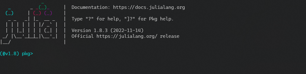
juliaWe will be presented with the Julia logo, as well as the version we’re using and some additional documentation information:
Output
We can exit the Julia REPL by typing exit().
Creating a Working Environment from the REPL
The first thing we’ll do before we install our packages is set up a working environment (similar to a Python virtual environment). For this, we will head to our working folder:
Code
cd computer-science/julia-for-beginnersWe will then access the Julia REPL and use the right bracket ] to access Julia’s pkg package manager. This will change the prompt and tell us which Julia version we’re currently using:
Pkg Prompt From The REPLWe will then type generate followed by our project_name:
Code
generate project_nameOutput
Generating  project julia_project:
	julia_for_beginners\Project.toml
	julia_for_beginners\src\julia_project.jl
This will create our environment folder containing two files:
Project.tomlwill contain the environmentname, the environmentUUID, theauthor, and the project version (not to be confused with the Julia version we’re using)julia_for_beginners.jlwill be our main project file (Julia files have the.jlextension). If we open our file, we can see that we have some information already there:
Code
module julia_project
greet() = print("Hello World!")
end # module julia_projectWe can then head back to VS Code, select File, Open Folder, and choose our environment folder. We can ensure we’re using the right environment by opening the VS Code command palette and selecting the Julia: Change Current Environment option. This will display all the Julia environments we have currently set up. We can select the environment name we just created, and it will automatically be set as default for this folder (if it has not already done so).
We can make a simple test by opening our julia_project.jl file, deleting the existing contents, typing some code, and executing it:
Code
println("This is our first Julia Project!!")Output
This is our first Julia Project!!We can then proceed to install some useful packages.
Installing packages using pkg from the REPL
Julia uses its own package manager called pkg. It’s installed by default on all Julia releases.
We may notice that once we’re inside pkg and inside our project folder, the environment is not active by default (the left prompt will display our current environment). Before installing our packages, we must activate our environment; otherwise, the packages will be installed in the global environment rather than in the one we just created. For this, we will type the following inside pkg:
Code
activate .Output
Activating new project at `C:\Users\username\Documents\computer-science\julia-for-beginners`We are now inside our environment and ready to start installing the packages we’ll use throughout this segment.
Installing packages in Julia is extremely simple. There are two main ways we can follow:
- We can directly use the
pkgpackage manager from the Julia REPL by typing the right bracket ] symbol. We can then install a package:
Code
add package_name- We can also call
pkgfrom within a Julia script or the Julia REPL without having to enterpkg:
Code
using Pkg
Pkg.add("Package Name")Note that for the first option, we don’t enclose our package_name in quotes, while with the second approach, we do need to enclose the package name in quotes.
Let us now install the DataFrames package directly from pkg inside the Julia REPL.
Code
add DataFramesOutput
Precompiling project...
  9 dependencies successfully precompiled in 37 seconds. 18 already precompiled.
Once we install our first package, a new file named Manifest.toml will be created. This file is important since it will contain all the currently installed packages, their dependencies, UUIDs and versions.
To install multiple packages at once, we can use a Julia script which calls Pkg and installs the required packages. We’ll create a new packages.jl file inside our environment. We will then include the following and run it:
Code
pkgs = ["DataFrames", "Plots", "CSV", "Pluto", "PlutoUI", "IJulia", "TypeTree"]

using Pkg

Pkg.add(pkgs)The following packages will be installed:
DataFramesPlotsCSVPlutoPlutoUIIJuliaTypeTree
This will take some time since Julia first needs to download the packages if we still don’t have them in our local machine and then precompile them.
In the end, we should get a similar output as the one below:
Output
66 dependencies successfully precompiled in 235 seconds. 396 already precompiled.We can test that our required packages were installed by closing the packages.jl script, going back to our julia_project.jl file, and loading a couple of random packages by using the using command. This imports our required packages and makes them available for our session:
Code
using DataFrames
using Plots

# Test libraries
x = range(0, 10, length=100)
y = sin.(x)
plot(x, y)

z = round.(y, digits=4)

print(z)Alternatively, we can also import our packages using commas ,:
Code
using DataFrames, Plots

# Test libraries
x = range(0, 10, length=100)
y = sin.(x)
plot(x, y)

z = round.(y, digits=4)

print(z)If everything goes well, the plot should appear on a new window. It can also be accessed by heading to the Julia Extension menu in the left panel and expanding the PLOT NAVIGATOR menu. We should have our first plot figure, plot_01. We can click on it, and it will display.
Output
[0.0, 0.1008, 0.2006, 0.2984, 0.3931, 0.4839, 0.5696, 0.6496, 0.723, 0.7889, 0.8469, 0.8962, 0.9364, 0.967, 0.9878, 0.9985, 0.999, 0.9893, 0.9696, 0.9399, 0.9007, 0.8523, 0.7952, 0.73, 0.6574, 0.5781, 0.4928, 0.4026, 0.3082, 0.2107, 0.1111, 0.0103, -0.0906, -0.1906, -0.2886, -0.3837, -0.4748, -0.5612, -0.6418, -0.7158, -0.7826, -0.8414, -0.8916, -0.9327, -0.9643, -0.9861, -0.9978, -0.9994, -0.9908, -0.972, -0.9434, -0.9051, -0.8576, -0.8014, -0.737, -0.6651, -0.5864, -0.5017, -0.412, -0.318, -0.2207, -0.1213, -0.0206, 0.0804, 0.1805, 0.2787, 0.3742, 0.4658, 0.5526, 0.6338, 0.7086, 0.7761, 0.8358, 0.8869, 0.9289, 0.9615, 0.9843, 0.9971, 0.9997, 0.9921, 0.9744, 0.9467, 0.9094, 0.8629, 0.8075, 0.7439, 0.6727, 0.5947, 0.5106, 0.4213, 0.3277, 0.2308, 0.1315, 0.0308, -0.0701, -0.1703, -0.2688, -0.3646, -0.4566, -0.544]
Plots PackageTo uninstall a package from our current environment, we can go to our environment’s Julia REPL and type the following:
Code
using Pkg
Pkg.rm("Symbolics")We can then confirm that our package has been removed, by opening our environment’s Project.toml file:
Output
code .\Project.tomlWe should not see the removed package nor its UUID referenced in the [deps] section.
If we are getting errors regarding unresolved dependencies, we can resolve them from our environment’s Julia REPL:
Code
using Pkg
Pkg.resolve()This command will rebuild our Manifest.toml file if a conflict is found.
When working with environments, the instantiate command is a handy tool. It will install all dependencies required for the project on Manifest.toml. In simpler terms, we can clone a Julia repository containing a Manifest.toml file and run this command; it will install all the packages required for the project.
We can execute this command directly from our environment’s Julia REPL:
Code
using Pkg
Pkg.instantiate()Getting familiar with the VS Code extension
Julia’s VS Code extension offers multiple functionalities:
- Syntax highlighting
- Snippets: latex and user-shared snippets
- Julia specific commands
- Integrated Julia REPL
- Code completion
- Hover help
- A linter
- Code navigation
- Tasks for running tests, builds, benchmarks and build documentation
- A debugger
- A plot gallery
- A grid viewer for tabular data
- Integrated support for
Weave.jl
The complete official documentation can be found here.
1. Using the Julia REPL inside VS Code
We can open a Julia REPL that already has our active environment by opening the VS Code command palette and selecting Julia: Start REPL. We can also do this directly by using the alt + j + o (Julia open) key combination. We can confirm that we’re using our current environment by entering into pkg using the right bracket ]; our environment will display on the REPL prompt. This method knows which Julia environment to use by looking at the Project.toml & Manifest.toml files inside our current folder. If it finds none, it will default to the global Julia environment.
We can directly run a script in the current environment REPL by using the ctrl + F5 key combination. To clear our REPL, we use the ctrl + l key combination. We can also directly input commands into the environment REPL, and they will run.
If we would like to run a single code selection, we can select the code we’d like to run and use the ctrl + shift key combination. This is very useful since we don’t have to run the entire script, as previously defined variables will not get deleted upon execution.
We can also run a Julia script directly from our Windows terminal inside VS Code. The catch is that we will need to specify an additional --project parameter for the correct environment REPL to execute our script. Otherwise, the script will be executed by the global Julia environment:
Code
julia --project .\julia_project.jl2. Workspace variables
We can view our workspace variables by heading to the Julia menu in the left panel, expanding the WORKSPACE tab, and expanding the Julia REPL tab. This tab will show us all the imported packages for the current session and all the defined variables.
Julia VS Code extension has a built-in variable visualizer similar to Spyder. We can access any object by clicking the table icon at the right of the variable we wish to visualize:
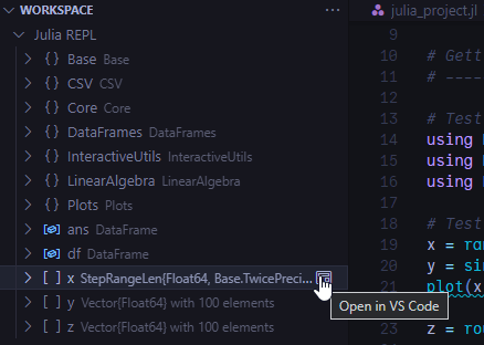
The beauty of this method is that it works for variables and tables.
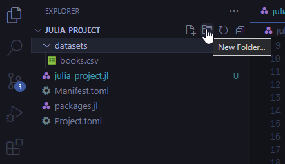
To illustrate this, we’ll create a very simple .csv file by heading to the EXPLORER tab on the left panel, clicking on New Folder…, and naming it datasets:
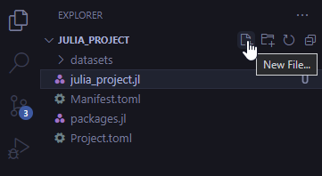
We’ll then create a .csv file inside our datasets folder, and name it test.csv:
We will open this file and populate it with the following:
Code
Name, Age, Occupation
John, 34, Scientist
Mary, 25, Astronaut
Paul, 27, WriterWe will now read the CSV file into a DataFrame object. We already have the two required packages installed, so we’ll only need to import them to our current session:
Code
using CSV, DataFrames

df_1 = CSV.read("datasets/test.csv", DataFrame)We can now head back to the Julia menu in the left panel, expand our WORKSPACE tab, and open our table in VS Code.
Output
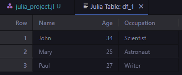
We can also display any figure in the VS Code viewer by using the following syntax inside our script:
Code
vscodedisplay(df_1)Upon execution, this method will automatically open our table in a new tab.
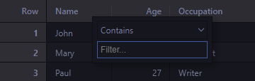
This table view has some nice features we can take advantage of to visualize and explore a newly imported data set quickly. We can search, sort and filter by using the navigation buttons on each column header:
Getting familiar with JupyterLab
As mentioned earlier, Julia supports two primary notebook environments: JupyterLab & Pluto.jl. JupyterLab is very popular among Data Scientists & Data Analysts and supports various languages.
If we recall the package installation segment above, we already added a package named IJulia to our environment. This package provides a Julia kernel for JupyterLab.
To launch a new JupyterLab session, we can open a new PowerShell instance, head to our working folder and open a new JupyterLab session:
Code
cd \julia_project

jupyter-labOutput
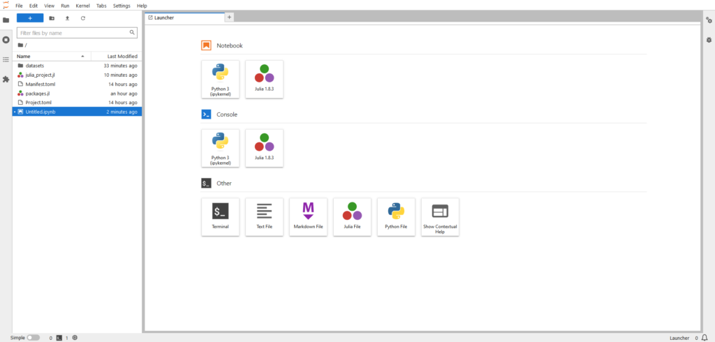
We can create a new Julia notebook, rename it as julia_project.ipynb and confirm that we started this session under our target working environment by importing a package we already installed:
Code
using CSVA detailed guide on using JupyterLab is out of the scope of this article. Still, the official documentation is extremely helpful for those looking to dive deeper into this awesome notebook environment.
Once our session and notebook are ready, we can practically use them as we would with any other programming language.
Getting familiar with Pluto.jl
The other notebook environment we will discuss in this article is Pluto.jl. It’s Julia-specific, extremely fun to use, has a minimal interface, and shares many similarities with JupyterLab.
Pluto can be installed using pkg. We can also complement our installation by getting the PlutoUI package; it will provide some additional html"<input>" functionalities. Since we already did this, we can head to our environment’s Julia REPL, and import the Pluto package:
Code
using PlutoWe will then run the package:
Code
Pluto.run()Upon execution, a new Pluto session will be created and launched in our system’s default browser:
Output
[ Info: Loading...
[ Info: Listening on: 127.0.0.1:1234, thread id: 1
┌ Info:
└ Opening http://localhost:1234/?secret=t6tEXgJ3 in your default browser... ~ have fun!
┌ Info:
│ Press Ctrl+C in this terminal to stop Pluto
└
Output
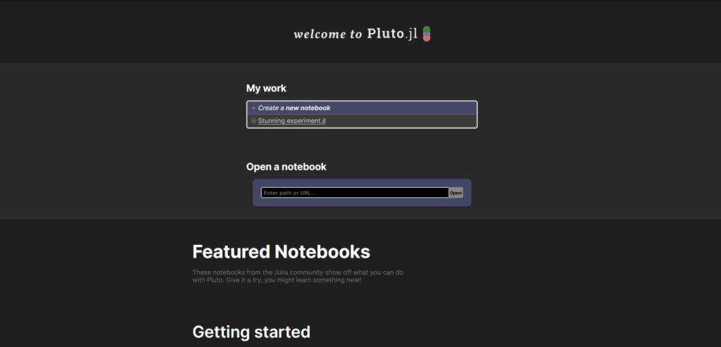
We will be presented with Pluto’s main menu, where we will create a new notebook by selecting the Create a new notebook option. We will name it julia_project_pluto.jl (it’s important to include the .jl extension).
As with JupyterLab, we will make sure we have installed Pluto in the correct environment:
Code
using PlutoUIAfter this command, we will need to restart our Pluto instance since it will reload with additional UI features enabled.
We can display the Shortcuts menu using the F1 shortcut. The relevant shortcuts we will use in this segment will be:
- Shift + Enter: Run cell
- Ctrl + Enter: Run cell and add cell below
- Del or Backspace: Delete empty cell
- Ctrl + C: Copy selected cells
- Ctrl + X: Cut selected cells
- Ctrl + V: Paste selected cells
- Ctrl + M: Toggle markdown
1. Writing multiple lines on a single cell
Unlike with JupyterLab, if we try to write multiple lines of code in a single cell and execute, Pluto will complain:
Code
x = "Hello"
b = "World"
println(x, b)Output
Multiple expressions in one cell.
How would you like to fix it?
- [Split this cell into 3 cells](http://localhost:1234/edit?id=5cff5130-afd3-11ed-18db-8554d52bda68#), or

- [Wrap all code in a _begin ... end_ block.](http://localhost:1234/edit?id=5cff5130-afd3-11ed-18db-8554d52bda68#)

1.  **top-level scope**@_none:1_
We need to wrap our code in a begin end statement:
Code
begin
	x = "Hello"
	b = "World"
	println(x, b)
endOutput
HelloWorldConversely we can include each new line in a different cell:
Code
d = "Hello"t = "World"println(d, t)Output
HelloWorld2. Inserting Markdown cells
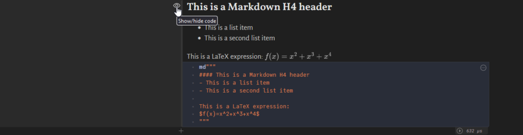
As with JupyterLab, Pluto supports Markdown cells. To insert a Markdown cell, we can add a new cell and use the ctrl + m keyboard shortcut:
Code
md"""
#### This is a Markdown H4 header
- This is a list item
- This is a second list item

This is a LaTeX expression:
$f(x)=x^2+x^3+x^4$
"""Output
This is a Markdown H4 header
- This is a list item
- This is a second list item
This is a LaTeX expression: 
We can hide the actual Markdown code and keep the output by using the eye icon at the left of any Markdown cell:
3. Using PlutoUI
We mentioned that PlutoUI brings interesting UI functionalities to a Pluto notebook.
We can display all of PlutoUI methods:
Code
varinfo(PlutoUI)Output
| name | size | summary |
|---|---|---|
| BuiltinsNotebook | 356.538 KiB | Module |
| Button | 144 bytes | DataType |
| CheckBox | 144 bytes | DataType |
| Clock | 184 bytes | DataType |
| ClockNotebook | 280.173 KiB | Module |
| ColorPicker | 40 bytes | UnionAll |
| ColorStringPicker | 144 bytes | DataType |
| ConfirmNotebook | 274.660 KiB | Module |
| CounterButton | 144 bytes | DataType |
| DateField | 160 bytes | DataType |
| DatePicker | 160 bytes | DataType |
| DownloadButton | 152 bytes | DataType |
| Dump | 152 bytes | DataType |
| FilePicker | 144 bytes | DataType |
| LabelButton | 144 bytes | DataType |
| LocalResource | 0 bytes | LocalResource (generic function with 1 method) |
| MultiCheckBox | 80 bytes | UnionAll |
| MultiCheckBoxNotebook | 280.652 KiB | Module |
| MultiSelect | 80 bytes | UnionAll |
| NumberField | 192 bytes | DataType |
| PasswordField | 144 bytes | DataType |
| PlutoUI | 650.302 KiB | Module |
| 0 bytes | Print (generic function with 1 method) | |
| Radio | 168 bytes | DataType |
| RangeSlider | 240 bytes | DataType |
| RangeSliderNotebook | 277.834 KiB | Module |
| RemoteResource | 256 bytes | DataType |
| Resource | 256 bytes | DataType |
| Scrubbable | 248 bytes | DataType |
| ScrubbableNotebook | 278.749 KiB | Module |
| Select | 152 bytes | DataType |
| Show | 80 bytes | UnionAll |
| Slider | 40 bytes | UnionAll |
| TableOfContents | 176 bytes | DataType |
| TableOfContentsNotebook | 284.140 KiB | Module |
| TerminalNotebook | 283.801 KiB | Module |
| TextField | 208 bytes | DataType |
| TimeField | 160 bytes | DataType |
| TimePicker | 0 bytes | TimePicker (generic function with 2 methods) |
| WebcamInput | 200 bytes | DataType |
| WebcamInputNotebook | 295.818 KiB | Module |
| WithIOContext | 40 bytes | UnionAll |
| as_html | 0 bytes | #4 (generic function with 1 method) |
| as_mime | 0 bytes | as_mime (generic function with 2 methods) |
| as_png | 0 bytes | #4 (generic function with 1 method) |
| as_svg | 0 bytes | #4 (generic function with 1 method) |
| as_text | 0 bytes | #4 (generic function with 1 method) |
| br | 20 bytes | HTML{String} |
| confirm | 0 bytes | confirm (generic function with 1 method) |
| with_terminal | 0 bytes | with_terminal (generic function with 1 method) |
3.1 Creating reactive buttons
We see that we have a Button method available. We can create a new button object and then assign a macro to it so that we can use it to interact with our notebook in multiple ways:
Let us define a button and bind it to a variable my_var:
Code
@bind my_var Button("We Love Julia")We can then define a code block which will contain our my_var variable, along with some actions to be executed:
Code
data = let
	my_var
	f = rand(2)
	println("🖤", round.(f, digits=4), "🖤")
endIf we execute the code above for the first time, our variable will be instantiated:
Output
🖤[0.7841, 0.4072]🖤We can now click on our defined button, and the cell will be referenced again, thereby running the code block we defined:
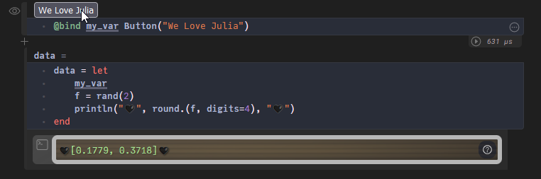
We can see that a new pair of random numbers was generated.
We can also create Radio buttons, which can be assigned to a macro that reactively displays information depending on the option selected:
Code
@bind writer Radio(["William Shakespeare", "Alexandre Dumas", "Victor Hugo"])println("Hi, I'm ", writer)When we select William Shakespeare, he properly introduces himself:
Output
Hi, I'm William ShakespeareAs we can imagine, there are many instances where these reactive objects could be useful. One such example would be flow control, where we could define breakpoints within a function. Another great application would be for debugging purposes, or we could also use buttons for dynamically displaying visuals.
Basic syntax
Now that we have some tools in our hands, we can start reviewing the basic Julia syntax. We will find many similarities with Python syntax; that’s because Python is extremely easy to write, and Julia inherited a wide range of syntactic elements from it.
For this section, we will create a new Pluto notebook and name it basic_syntax.jl.
1. Comments
As with Python, we can define single-line or multiline comments:
Code
# This is a single-line comment

#=
This is a multiline comment
=#We can also define comments after a variable definition:
Code
my_var = 3.1416 # This is Pi2. Variables
We can define variables by using the equal = sign:
Code
begin
	# Assigning integer
	x = 10

	# Assigning string types
	y = "Hello World"

	# Assigning float types
	z = -3.1416

	# Using a Unicode character as variable name
	λ = 30

	println(x)
	println(y)
	println(z)
	println(λ)
endOutput
10
Hello World
-3.1416
30
We need to be careful when assigning variables; e.g. if we define the + operator as a new variable, we will overwrite the actual Base:.+ method and start getting all kinds of errors, additional to being extremely hard to debug. We must remember reserved characters since Julia will not throw errors if we reassign them.
If we messed up and assigned a reserved name to a variable, we can reset it to its Base method:
Code
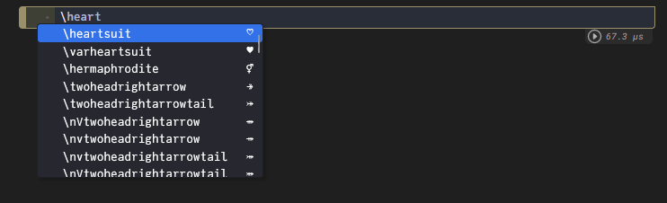
+ = Base.:+If we recall, we can use Unicode characters as variable names in Julia. Of course, it’s tedious to always refer to a Unicode character cheat sheet and copy and paste the required character. With Julia, we can simply use the backslash \ character followed by the character name we’re looking for and hit TAB. This will automatically insert the Unicode character:
Code
\lambdaOutput
λThe character names are equivalent to LaTeX names, so if we’re already familiar with LaTeX syntax, we should feel right at home.
If we’re unsure about a specific character’s name, we can start typing the name that would make more sense and then hit TAB. Pluto will display the entire list of available characters, where we can select the one we’re looking for:
We can also assign multiple variables using a single line:
Code
γ, θ = 300, 200println(γ, " + ", θ)Output
300 + 2003. Print statements
There are multiple methods we can use to print in Julia. The two most used are:
printprintln
3.1 print
The print statement will print to stdout without a newline in between, even if we specify the statements in two separate lines of code:
Code
π, ℯ = 3.1416, 0.5772begin
print(π)
print(ℯ)
endOutput
3.14160.57723.2 println
In contrast, the println method (print line) will include a newline at the end of each call:
Code
begin
	println(π)
	println(ℯ)
endOutput
3.1416
0.5772
There are more printing methods available, but we’re not going to dive deeper since the two we mentioned will suffice for almost any situation.
4. Data types
Julia’s type system is dynamic but gains some of the advantages of static type systems by making it possible to indicate that certain values are of specific types.
Julia has a wide variety of types, which can be classified into supertypes or subtypes, depending on the hierarchy of our data type.
We can view Julia’s Signed types in an ASCII tree-like structure by using the TypeTree.jl package:
Code
using TypeTreeprint(join(tt(Signed), ""))Output
Signed
 ├─ BigInt
 ├─ Int128
 ├─ Int16
 ├─ Int32
 ├─ Int64
 └─ Int8
We can go even higher in the tree structure and display all Number subtypes:
Code
print(join(tt(Number), ""))Output
Number
 ├─ Complex
 └─ Real
     ├─ AbstractFloat
     │   ├─ BigFloat
     │   ├─ Float16
     │   ├─ Float32
     │   └─ Float64
     ├─ AbstractIrrational
     │   └─ Irrational
     ├─ Integer
     │   ├─ Bool
     │   ├─ Signed
     │   │   ├─ BigInt
     │   │   ├─ Int128
     │   │   ├─ Int16
     │   │   ├─ Int32
     │   │   ├─ Int64
     │   │   └─ Int8
     │   └─ Unsigned
     │       ├─ UInt128
     │       ├─ UInt16
     │       ├─ UInt32
     │       ├─ UInt64
     │       └─ UInt8
     └─ Rational
We can also display all the subtypes belonging to the Any supertype. We will truncate the output since there are too many entries to fit in one code block:
Code
print(join(tt(Any), ""))Output
Any
 ├─ AbstractArray
 │   ├─ AbstractRange
 │   │   ├─ LinRange
 │   │   ├─ OrdinalRange
 │   │   │   ├─ AbstractUnitRange
 │   │   │   │   ├─ Base.IdentityUnitRange
 │   │   │   │   ├─ Base.OneTo
 │   │   │   │   ├─ Base.Slice
 │   │   │   │   └─ UnitRange
 │   │   │   └─ StepRange
 │   │   └─ StepRangeLen
 │   ├─ Base.ExceptionStack
 │   ├─ Base.LogicalIndex
 │   ├─ Base.MethodList
 │   ├─ Base.ReinterpretArray
 │   ├─ Base.ReshapedArray
 │   ├─ Base.SCartesianIndices2
 │   ├─ BitArray
 │   ├─ CartesianIndices
 │   ├─ Core.Compiler.AbstractRange
 │   │   ├─ Core.Compiler.LinRange
 │   │   ├─ Core.Compiler.OrdinalRange
 │   │   │   ├─ Core.Compiler.AbstractUnitRange
 ...
There are multiple data types in Julia. We will only review the most used ones:
4.1 Integer types
Julia has a total of 10 integer subtypes, where 5 of them are signed, and 5 are unsigned:
| Type | Signed? | Number of bits | Smallest value | Largest value |
|---|---|---|---|---|
Int8 | ✓ | 8 | -2^7 | 2^7 – 1 |
UInt8 | 8 | 0 | 2^8 – 1 | |
Int16 | ✓ | 16 | -2^15 | 2^15 – 1 |
UInt16 | 16 | 0 | 2^16 – 1 | |
Int32 | ✓ | 32 | -2^31 | 2^31 – 1 |
UInt32 | 32 | 0 | 2^32 – 1 | |
Int64 | ✓ | 64 | -2^63 | 2^63 – 1 |
UInt64 | 64 | 0 | 2^64 – 1 | |
Int128 | ✓ | 128 | -2^127 | 2^127 – 1 |
UInt128 | 128 | 0 | 2^128 – 1 | |
Bool | N/A | 8 | false (0) | true (1) |
We can define a variable and declare it as Int32 type by using double colon :: after the variable definition:
Code
d::Int64 = 1000We can verify the variable type by using the typeof method:
Code
typeof(d)Output
Int64We can also test if our variable is of a specific type, by using the isa operator:
Code
d isa Int64Output
trueWe can convert or promote an existing variable data type to a different type using the convert method if required. In this example, we convert from Int64 to its unsigned version:
Code
δ = convert(UInt64, d)Output
δ = 0x00000000000003e84.2 Floating-point types
Julia has three different floating-point types depending on the maximum number of accepted bits:
| Type | Precision | Number of bits |
|---|---|---|
Float16 | half | 16 |
Float32 | single | 32 |
Float64 | double | 64 |
We can define a new variable and set its type to Float64, even if our initial declaration doesn’t have decimal precision:
Code
g::Float64 = 1000gOutput
1000.04.3 Binary and octal types
Julia also supports binary and octal systems. We can declare a variable and then cast it to its binary form:
Code
begin
	β = 7
	typeof(β)
endOutput
Int64Code
β_1 = bitstring(β)Output
β_1 = "0000000000000000000000000000000000000000000000000000000000000111"4.4 String and Character types
4.4.1 String types
String types are defined by enclosing the value in double quotes "":
Code
σ = "This is the greek letter sigma"Note that we mentioned double quotes "" and not single quotes ''. This is because, unlike Python, single quotes are used to define characters and not strings. We’ll discuss character objects in a moment.
Code
typeof(σ)Output
StringAs with Python, we can index a string and return a substring:
Code
σ[13:17]Output
"greek"We can also index a single element, but the returned object will be of a different type:
Code
σ[1]Output
'T': ASCII/Unicode U+0054 (category Lu: Letter, uppercase)Instead of returning a String type, this operation returned a character type.
Code
typeof(σ[1])Output
Char4.4.2 Character types
Character objects (Char) are 32-bit primitive data types. They have a special literal representation and appropriate arithmetic behaviour. They can also be converted into numeric values representing a Unicode code point.
We can define a Char by using single quotes '':
Code
my_char = 'π'Output
my_char = 'π': Unicode U+03C0 (category Ll: Letter, lowercase)This tells us the Unicode representation for π. If we perform a Google Search, we can see that, in fact, U+03C0 is the Unicode representation of π.
Unicode characters can also be represented numerically. We can convert a Char object to its Int representation:
Code
begin
	my_int_char = '?'
	println(my_int_char)
	println(typeof(my_int_char))
	my_int_char = Int(my_int_char)
	println(my_int_char)
	println(typeof(my_int_char))
endOutput
?
Char
63
Int64
If we perform a Google Search, we can see that the numeric representation of the ? Unicode character is, in fact, 63, and our new data type is Int64.
We can convert our numerical representation back to a Char type by performing the inverse operation:
Code
Char(my_int_char)Output
'?': ASCII/Unicode U+003F (category Po: Punctuation, other)We can use multiple string & character methods such as unions, concatenations, interpolations, repetitions, conversions, and advanced regex techniques. We will not explore all the possibilities; the complete documentation can be consulted here.
4.5 Boolean types
Boolean types can be defined by using lowercase letters:
Code
begin
	b = true
	t = false
endCode
begin
	println(typeof(b))
	println(typeof(t))
endOutput
Bool
Bool
In Julia, Bool is a subtype of Integer; true equals 1, while false equals 0. We can do numerical operations on Bool types without the need for any type conversion:
Code
b - 1Output
05. Native data structures
Julia has several native data structures. They are abstractions of data that represent some form of structured data. We will cover the most used ones. There are also multiple data structures not native to Julia, such as DataFrames and SparseArrays, but we won’t be covering those here.
5.1 Tuples
A tuple is a fixed-length container that can hold multiple different types. It’s an immutable object, meaning it cannot be modified after its instantiation.
To construct a tuple, we can use parentheses () to delimit the beginning and end, along with commas , as delimiters between values:
Code
my_tuple = (1, "2", '3', "four", "🚀")Output
my_tuple = (1, "2", '3', "four", "🚀")We can index a tuple by using brackets []:
Code
my_tuple[5]Output
"🚀"What we cannot do, is mutate a tuple object:
Code
my_tuple[5] = λOutput
MethodError: no method matching setindex!(::Tuple{Int64, String, Char, String, String}, ::Int64, ::Int64)
    top-level scope@Local: 1[inlined]
We can iterate over the items of a tuple (we’ll cover for loops in more detail soon enough):
Code
for i in my_tuple
	println(i)
endOutput
1
2
3
four
🚀
There’s also a special type of tuple called NamedTuple. We will not cover it here, but it can be consulted in the official documentation.
5.2 Ranges
A range in Julia represents an interval between start and stop boundaries. We can define a range by using the start:stop syntax:
Code
my_range = 1:7Output
my_range = 1:7We can index a range and iterate over its elements:
Code
begin
	my_range_2 = 1:7
	println(my_range_2[7])

	for i in my_range_2
		println(i)
	end
endOutput
7
1
2
3
4
5
6
7
We can also build an array comprehension (similar to Python’s list comprehensions) by using a range in combination with a for loop, all enclosed in brackets []:
Code
begin
	my_array_comp = [x for x in 1:7]
	println(my_array_comp)
endOutput
[1, 2, 3, 4, 5, 6, 7]5.3 Arrays
In Julia, there are no list objects as in Python. We instead have arrays. They are mutable, can be one-dimensional or multi-dimensional, and can hold multiple objects.
There are two main array subtypes in Julia:
- Vectors
- Matrices
5.3.1 Vectors
Vectors are one-dimensional objects that can be defined using brackets:
Code
my_vector = [1, 2, 3]If we take a look at our my_vector data type, we can see that we have a Vector containing Int64 objects:
Code
typeof(my_vector)Output
Vector{Int64} (alias for Array{Int64, 1})We can also declare a mixed-type Vector object:
Code
begin
	my_vector_2 = [1, 2, "3"]
	typeof(my_vector_2)
endOutput
Vector{Any} (alias for Array{Any, 1})When no supertype is given, the default one is Any – a predefined abstract type that all objects are instances of and all types are subtypes of. In type theory, Any is commonly called “top” because it is at the apex of the type graph.
5.3.2 Matrices
We can declare matrices in multiple ways.
We can use a collection of vectors nested inside brackets [] (it’s important to note that, unlike Python, we’re not using commas to separate each vector):
Code
begin
	my_matrix = [[1, 2] [3, 4] [5, 6]]
	println(typeof(my_matrix))
	println(my_matrix)
endOutput
Matrix{Int64}
[1 3 5; 2 4 6]
We can also declare a matrix of undefined values by specifying it’s dimensions and content’s data type:
Code
begin
	my_matrix_2 = Matrix{Float64}(undef, 4, 2)
	println(typeof(my_matrix_2))
	println(my_matrix_2)
endOutput
Matrix{Float64}
[0.0 0.0; 0.0 0.0; 0.0 0.0; 0.0 0.0]
In Linear Algebra, it’s common to use matrices of ones and zeros:
Code
begin
	my_matrix_zeros = zeros(4, 2)
	my_matrix_ones = ones(4, 2)
	println(my_matrix_zeros)
	println(my_matrix_ones)
endOutput
[0.0 0.0; 0.0 0.0; 0.0 0.0; 0.0 0.0]
[1.0 1.0; 1.0 1.0; 1.0 1.0; 1.0 1.0]
It’s also common to specify matrices of random values. We can do so by using the Base rand method:
Code
rand(5,5)Output
5×5 Matrix{Float64}:
 0.685521  0.667868  0.368505  0.579188  0.67113
 0.869676  0.477044  0.576164  0.717674  0.348186
 0.163335  0.257388  0.841889  0.469516  0.409196
 0.253942  0.527152  0.808858  0.800833  0.609731
 0.4401    0.718082  0.748828  0.284882  0.410565
This method will return a matrix of dimension n×n, with Float64 type values between 0 and 1.
If we would like to explore our matrix objects in more detail, we can employ dimension methods:
Code
begin
	my_matrix_rand = rand(5,5)
	println(length(my_matrix_rand))
	println(ndims(my_matrix_rand))
	println(size(my_matrix_rand))
endOutput
25
2
(5, 5)- The
lengthmethod will return the total number of elements in our matrix. - The
ndimsmethod will return the number of dimensions. - The
sizemethod will return our matrix’s size in row-column notation.
Finally, we can index our matrix similar to indexing other objects such as tuples or vectors:
Code
my_matrix_rand_2 = rand(2,5)begin
println(my_matrix_rand_2[1])
println(my_matrix_rand_2[2, 1])
println(my_matrix_rand_2[end])
endOutput
0.9069052054266634
0.4401923900688668
0.8721676196514414my_matrix_rand_2[1]will return the first element of our matrix.my_matrix_rand_2[2, 1]will return the element located in the second row, first column.my_matrix_rand_2[end]will return the last element in our matrix. Thebeginmethod can also be used to get the first element.
Arrays are the base for linear algebra in Julia and many other languages such as Python (by using np.arrays). This is why there is a multitude of different methods we can use to manipulate these objects. We will not cover them in detail but can be consulted on the Julia’s official documentation page.
5.4 Pairs
Pairs hold two objects which typically belong to each other. They are similar to Python’s dictionaries but are limited to one pair of objects. Pairs are specifically used in broadcasting operations, which we’ll review later on.
We can define a Pair by using the following notation:
Code
my_pair = "My Number" => 7We can access a Pair’s elements by using the first and last methods:
Code
begin
	println(first(my_pair))
	println(last(my_pair))
endOutput
My Number
7
5.5 Dicts
Dicts are mappings from keys to values. By mapping, we mean that if you give a Dict some key, the Dict can tell us which value belongs to that key. Dicts are mutable and accept multiple objects.
We can define a Dict using the following syntax:
Code
my_dict = Dict("ONE" => 1, "TWO" => 2, "THREE" => 3)Typically, keys are denoted by string type objects and have to be unique within a given Dict. If we accidentally define duplicated keys, Julia will keep the latter and discard the previous definition:
Code
begin
	my_dict_2 = Dict("ONE" => 1, "ONE" => 2, "THREE" => 3)
	println(my_dict_2)
endOutput
Dict("ONE" => 2, "THREE" => 3)Similar to Python, we can retrieve a given value by referring to its key:
Code
my_dict["ONE"]Output
1 We can also substitute a given value inside our Dict object:
Code
begin
	my_dict["ONE"] = 7
	println(my_dict)
endOutput
Dict("ONE" => 7, "THREE" => 3, "TWO" => 2)As we can see, this is an in-place operation that will mutate our Dict object.
We can also iterate over key-value pairs by using a for loop:
Code
for i in my_dict
	println(i)
endOutput
"ONE" => 7
"THREE" => 3
"TWO" => 2
We can do the same, but this time, extracting key-value pairs separately:
Code
for (i, j) in my_dict
    println(i, " => ", j)
endOutput
ONE => 7
THREE => 3
TWO => 2
6. Mathematical operators
Mathematical operators in Julia work very similarly to Python’s. We can consult the complete set by heading to the official documentation page.
| Expression | Name | Description |
|---|---|---|
+x | unary plus | the identity operation |
-x | unary minus | maps values to their additive inverses |
x + y | binary plus | performs addition |
x - y | binary minus | performs subtraction |
x * y | times | performs multiplication |
x / y | divide | performs division |
x ÷ y | integer divide | x / y, truncated to an integer |
x \ y | inverse divide | equivalent to y / x |
x ^ y | power | raises x to the yth power |
x % y | remainder | equivalent to rem(x,y) |
We can perform any mathematical operation using the following syntax:
Code
begin
	my_num_1 = 7
	my_num_2 = 2
	my_vec_1 = [3, 4, 5]
	println(my_vec_1 * my_num_1)
endOutput
[21, 28, 35]We can also use the updating operator forms for each case above. These operators update our variable without the need to redefine it:
| Expression | Name | Description |
|---|---|---|
x += y | binary plus | performs addition |
x -= y | binary minus | performs subtraction |
x *= y | times | performs multiplication |
x /= y | divide | performs division |
x ÷= y | integer divide | x / y, truncated to an integer |
x \= y | inverse divide | equivalent to y / x |
x ^= y | power | raises x to the yth power |
x %= y | remainder | equivalent to rem(x,y) |
7. Flow control
Flow control in Julia can be achieved by using multiple built-in methods. The most popular are:
- Logical operators
- Conditionals
ForloopsWhileloops
7.1 Logical operators
There are six basic logical or comparison operators in Julia:
| Expression | Name |
|---|---|
== | equality |
!=, ≠ | inequality |
< | less than |
<=, ≤ | less than or equal to |
> | greater than |
>=, ≥ | greater than or equal to |
We can perform a logical comparison by using the following syntax:
Code
begin
	e = 1
	f = 2
	println(e>f)
endOutput
false7.2 Conditionals
A complete Julia conditional evaluation includes 4 parts:
ifelseifelseend
We can either stick with just the if end statement combination if we have only one condition to evaluate or include the whole structure:
Code
begin
	for i in 1:10
		if i%2 != 0
			println("Odd number")
		else
			println("Even number")
		end
	end
endOutput
Odd number
Even number
Odd number
Even number
Odd number
Even number
Odd number
Even number
Odd number
Even number
7.3 For loops
We have already seen some for loop examples; they are very similar to their Python counterpart, except that we don’t require a colon : at the end of the statement, and we need to add an end statement at the end of our declaration:
Code
begin
	for i in 0:9
		println(i+1)
	end
endOutput
1
2
3
4
5
6
7
8
9
10
7.4 While loops
Similarly, we can define a while loop by using the syntax below
Code
begin
	i = 7

	while i >= 1
		println(i)
	    i -= 1
	end
endOutput
7
6
5
4
3
2
1
8. Functions
Functions in Julia, as in many other languages, are essential. Functions are similarly implemented in Julia compared to Python. Still, they have many additional features, such as broadcasting and native multiple dispatch support, which expand their functionality in ways Python simply can’t by default.
8.1 Defining a function
We can define a function by using the following syntax:
Code
function my_fun(x,y)
	   x + y
endOutput
my_fun (generic function with 1 method)We can then call our function:
Code
begin
	call_to_fun = my_fun(1, 2)
	println(call_to_fun)
endOutput
3Even though we did not include a return statement, our function will return the output of the only method available inside of it.
We can define our function in a more compact form:
Code
my_fun_2(x,y) = x + ySince, as we have mentioned, Julia accepts Unicode characters as part of its syntax, we could even write our own sum function:
Code
∑(x,y) = x + yWe can call it just as we would any other function:
Code
∑(7, 7)Output
14This non-return method works when we have one single value we would like to return, but we may also want to return multiple values:
Code
function my_fun_3(x, y)
	a = x*y
	b = x+y
	return a, b
endWe can then call our function:
Code
println(my_fun_3(7, 7))Output
(49, 14)We can of course declare nested functions, thus expanding the functionality of our parent function.
8.2 Broadcasting
Broadcasting is an extremely powerful concept in Julia, especially when performing vector & matrix operations. It lets us broadcast operations over the elements of the input objects. Broadcasting can be achieved using the dot . operator, which applies to any function or arithmetic operation.
We can define a function my_fun_b that will take a matrix as input, square each of its elements, and return the result.
We will first start by creating a matrix and an Int variable that will serve as inputs:
Code
my_matrix_b = rand(4, 4)We can then define our function my_fun_b:
Code
function my_fun_b(x)
	return x^2
endIf we call our function with my_matrix_b as its argument without broadcasting, we will get the squared matrix ( ) as a result, and not the element-wise operation:
Code
display(my_fun_nb(my_matrix_b))Output
4×4 Matrix{Float64}:
 1.26661   0.519347  1.13055   1.23636
 2.17724   1.23979   1.87389   1.73158
 0.63514   0.201745  0.51771   0.589747
 0.809722  0.554337  0.859173  0.652899
This is not what we’re looking for. Instead, we can use the broadcasting operator when calling our function. The dot . operator will go just after our function call and before the opening parenthesis ( for our arguments:
Code
display(my_fun_nb.(my_matrix_b))Output
4×4 Matrix{Float64}:
 0.896748   0.0097358    0.165206  0.648777
 0.812765   0.904707     0.794022  0.309314
 0.198626   0.000761553  0.113611  0.094145
 0.0153391  0.158666     0.417942  0.133245
We can see that we now get the result we were looking for.
8.3 Functions with a bang !
The bang ! symbol in Julia is used to differentiate mutating vs non-mutating operations. When we call a method along with !, it will mutate our input variable.
We can use the sort() method as example:
Code
begin
	my_vec_a = [1, 4, 5, 8, 3, 0]
	println(sort(my_vec_a))
	println(my_vec_a)
endOutput
[0, 1, 3, 4, 5, 8]
[1, 4, 5, 8, 3, 0]
As we can see, the way we called our function did not mutate the original structure of my_vec_a.
If we want to mutate it, we can usesort!() instead of sort():
Code
begin
	my_vec_b = [1, 4, 5, 8, 3, 0]
	println(sort!(my_vec_b))
	println(my_vec_b)
endOutput
[0, 1, 3, 4, 5, 8]
[0, 1, 3, 4, 5, 8]
Next steps
We covered a tiny sample of what Julia can do. This language has endless potential and can be used by many professionals and enthusiasts looking for a high-performance, bleeding-edge alternative to the current options.
Now that we know the basics of the Julia programming language, there are multiple paths we can choose to follow:
- Data Science & Machine Learning: Julia for Data Scientists would be a great next step for those interested in using this language for big data processing & parallelization, Machine Learning algorithm design & deployment, statistical analysis, and more.
- Optimization: Julia for Optimization and Learning imparted by the Czech Technical University in Prague, provides excellent introductory material for those interested in Optimization & Machine Learning techniques.
- Linear Algebra: Julia stands up when performing linear algebra-related operations. There is a huge collection of packages and documentation available. A great first step would be Basic Linear Algebra in Julia, imparted by the extremely well-versed Dr. Jane Herriman.
- Integral & Differential Calculus: No scientific language is complete without a robust set of calculus methods, and Julia, of course, is no exception. There is a great series of articles by jverzani aiming to cover the basics of calculus using Julia, ranging from simpler undergraduate concepts to more intermediate topics.
- Documentation: Julia can also be used for documentation purposes. In particular, the
Documenter.jlpackage offers excellent capabilities to write in Markdown offering a simple and easy-to-understand interface.
Conclusions
In this segment, we installed the Julia programming language from scratch along with Visual Studio as an IDE and the Visual Studio Julia extension as a handy tool. We also reviewed two great notebook environment options: JupyterLab and Pluto.jl.
Once we had our installations ready, we learned to use the Julia REPL from the Windows Terminal and from within VS Code using the Julia extension. We also learned how to create project environments, install packages within our environment, manage them appropriately, and write our first Julia program.
Finally, we introduced some of Julia’s core concepts, accompanied by hands-on examples using Pluto.jl and PlutoUI.
Julia is a language that has been gaining consistent popularity throughout the last few years. It was introduced as a fresh approach to scientific programming and is sure to become a building block for aspiring Data Scientists in the near future. It has so many innovative features that it’s hard to look the other way and continue using the well-established Data Science languages we have been using for several years.
Julia allows us to stop and think if what we’re doing and how we’re doing it is the most optimal way. It’s an ambitious project that aims to change how we look at high-performance scientific computing.
One thing to consider is that Julia is fast-evolving; each iteration brings on new changes, which might be small but can also consist of a complete refactoring of base functionality. This is critical because a library that worked yesterday with a given syntax might not work the same way today. Still, this is always part of the process of any programming language, and really, the most exciting one; witnessing a group of passionate people build the foundations for the future is always inspiring.