Machine Learning is a field focused on developing, comprehending, and utilizing computer programs that can learn from experience to model, predict, or control certain outcomes. This discipline has gained considerable traction in recent years as it has transformed how we approach problem-solving. Machine Learning algorithms can analyze vast amounts of data and produce more accurate results faster than hard-coded methods in some cases. Before Machine Learning, creating solutions to problems involved hard-coding solutions that accounted for every variable and parameter, which became increasingly difficult as the amount of data generated increased.
Machine Learning is a permanent fixture in the technology landscape, and it is beneficial to have a general understanding of the technology to appreciate its potential applications. As a result of this discipline, a variety of models can be applied to different applications. These applications range from product recommendations to image, speech, text recognition, sentiment analysis, DNA sequencing, global warming modelling, and temperature prediction. The potential applications of Machine Learning are vast, and almost every field of study has at least one problem where Machine Learning models can help create more efficient solutions.
In this article, we will discuss the different Machine Learning algorithm types using three different categorization methods. We will also qualitatively compare different Machine Learning models to grasp a generalized understanding. We will conclude this segment with some next steps for those interested in diving deeper into this exciting discipline.
We will not discuss each model in detail since there are too many to cover in one segment. There’s a dedicated 3-segment hands-on Guided Project, Exploratory Data Analysis, where we cover all the major classification algorithms along with a detailed comparison by using an example applied on medical data. There will also be future content covering diverse ML model implementations in detail.
We’ll be using Python scripts which can be found in the Blog Article Repo.
Machine Learning vs traditional programming
What’s so special about it? Why was it such a significant breakthrough in how we think of problem-solving? To explain this, we have to refer to how traditional computation is done.
Traditional computer programming has been around for over a century, with the first known computer program dating back to the mid-1800s. It refers to any manually created program that uses input data and executes it to produce the output; a programmer creates the program, but without anyone programming the logic, one has to formulate rules manually (this is what we’ll be referring to as hard-coding).
For example, we can define a function that will do a specific task based on a set of logical rules we explicitly describe. In this case, our function accepts a DataFrame object as input, evaluates each row of the age column, and performs a mathematical operation based on each age value:
Code
# Import modules
import pandas as pd

# Example 1: Hard-coded function

# Declare entries
p0 = ['Sarah', 'Howard', 22, 'Secretary', 1300]
p1 = ['John', 'Moore', 32, 'Illustrator', 3000]
p2 = ['Laszlo', 'Kreizler', 35, 'Alienist', 3500]
p3 = ['Willem', 'Van Bergen', 31, 'Pampered Child', 50000]
p4 = ['Libby', 'Hatch', 30, 'Nurse', 1100]
p5 = ['Lucifer', 'Morningstar', 35, 'Club Owner', 100000]
p6 = ['Chloe', 'Decker', 34, 'Detective', 1400]
p7 = ['Dan', 'Espinoza', 36, 'Detective', 1300]
p8 = ['Mazikeen', 'Smith', 35, 'Bounty Hunter', 20000]
p9 = ['Laura', 'Palmer', 22, 'Student', 100]
p10 = ['Dale', 'Cooper', 36, 'FBI Agent', 1800]
p11 = ['Harry', 'S. Truman', 34, 'Sheriff', 1300]
p12 = ['Bobby', 'Briggs', 23, 'Student', 80]
p13 = ['Gordon', 'Cole', 55, 'FBI Agent', 2000]

# Create list of lists
people_list = [p0, p1, p2, p3, p4,
               p5, p6, p7, p8,
               p9, p10, p11, p12,
               p13
               ]

# Declare DataFrame
df = pd.DataFrame(people_list,
                  columns = ['Name', 'Surname', 'Age', 'Job Position', 'Salary'])

# Declare function
def myFun(df):
    '''
    Parameters
    ----------
    df : Pandas DataFrame
        Contains 3 columns: Name, Surname, Age, Job Position, Salary (monthly in USD).

    Returns
    -------
    top_jobs : List
        Contains the top 7 paid job positions for a person between
        25 and 40 years old, sorted by importance.
    '''

    df_top = (df.query("`Age` >= 25 and `Age` <= 40").
              groupby('Job Position')['Salary'].mean().
              reset_index(name ='Average Salary').
              nlargest(7, 'Average Salary').
              sort_values(by='Average Salary', ascending=False).
              reset_index(drop=True)
              )

    return df_top

# Call function with df
print(myFun(df))Output
     Job Position  Average Salary
0      Club Owner        100000.0
1  Pampered Child         50000.0
2   Bounty Hunter         20000.0
3        Alienist          3500.0
4     Illustrator          3000.0
5       FBI Agent          1800.0
6       Detective          1350.0
Apart from the fact that being a club owner or a pampered child could be the key in life, we can see that this method implementation worked because we defined logical rules denoted by our query statements. These were explicitly stated and required logical reasoning behind the curtains.
This was also feasible because we had a very limited set of rules: age and Average Salary, which we used as features to return an output.
The problems surface when we have an extensive and potentially un-normalized set of features we need to consider, or even worst; we don’t know which ones could be leveraged to get the insight we’re looking for.
In Machine Learning, the algorithm automatically formulates the rules from its input and outputs a model we can use to perform predictions, classifications, or control.
These algorithms can go from extremely simple to extremely complex; it all depends on what we’re trying to solve, the input dimensions, and the complexity of our data set.
It’s important to remember that, as grandiose as it may seem, ML is just another tool in a very extensive toolbox; it’s easy to assume that ML can be applied to every possible problem and outperform any traditional algorithm, but the truth is, it does not substitute hard-coding entirely, nor does it do magic.
As with any tool, it has its applications and limitations and is based on rigorous mathematical and statistical theory. In fact, Machine Learning can be thought of as a combination of probability theory, statistics & optimization. We’ll see why in a moment.
The core concepts of Machine Learning
As we already mentioned, ML algorithms build models based on sample data, known as training data, to make predictions or decisions without being explicitly programmed to do so.
When deploying an ML model, we must consider how we will represent the knowledge, decide if our model is a good fit for our particular case, and optimize our model to return the most optimal answer.
These steps apply to any ML algorithm deployment process and can be summarized as follows:
- Representation: What the model looks like; how knowledge is represented.
- Evaluation: How good models are differentiated; how programs are evaluated .
- Optimization: The process for finding good models; how programs are generated.
Every model works differently, meaning the mathematical & statistical theory behind may differ. Still, they all follow a generalized set of steps to provide a solution to the problem we define:
- Data Collection: Collect relevant data for the problem we’re trying to solve. This can be from existing datasets or by collecting new data.
- Data Preparation: Clean and preprocess the data to remove any irrelevant or inconsistent data points, handle missing values, and transform the data into a format suitable for analysis.
- Feature Selection/Extraction: Select or extract the most important features from the data relevant to the problem we’re trying to solve. This step is crucial because it can significantly impact the model’s performance.
- Model Selection: Choose an appropriate machine learning algorithm for the problem we’re trying to solve. This involves understanding the characteristics of the data, the type of problem we’re trying to solve, and the desired output.
- Model Training: Train the model on the data to learn the patterns and relationships between the input features and the target variable. This involves selecting appropriate hyperparameters and using optimization techniques to minimize the error between the predicted and actual values.
- Model Evaluation: Evaluate the model’s performance on a separate dataset not used for training. This helps to ensure that the model is not overfitting to the training data and can generalize well to new data.
- Model Tuning: Fine-tune the model by adjusting hyperparameters or trying different algorithms to improve its performance on the evaluation dataset.
- Deployment: Deploy the model in a production environment and integrate it into a more extensive system to make predictions on new data. This involves considerations such as model versioning, monitoring, and security.
Finally, we have several ways to classify the different types of ML models. The classification methods depend on the following:
- How they learn
- How they represent data associations
- How they conceptualize a potential solution
Classification by learning techniques
Machine Learning algorithms can be classified by how they learn. There are three main types and some other subclassifications:
- Supervised Learning
- Unsupervised Learning
- Reinforcement Learning
1. Supervised Learning
Supervised Learning is a machine learning approach that employs labelled datasets to train algorithms that can accurately classify data or forecast outcomes. A labelled dataset can be viewed as data with tags that define what the data represents.
If we look at our previous example, we used a DataFrame with five columns:
Code
print(df.columns)Output
Index(['Name', 'Surname', 'Age', 'Job Position', 'Salary'], dtype='object')This means that our data is labelled; it has identifiable tags which we can use to make sense of the information it presents.
More specifically, in the Machine Learning context, a label is the specific vector we’re trying to predict or use to classify. This depends on the problem we’re trying to solve.
For example, we could use our DataFrame df to train a model which predicts a person’s Salary based on other attributes such as Age and Job Position. These attributes would be called features, and the target to predict, in this case, Salary, would be our label. We could solve this problem either by regression or classification; these are the two main subclasses of Supervised Learning.
1.1 Regression
Regression is most commonly known since it’s taught very early in math courses and has multiple applications, from market analysis to financial analysis to trend forecasting. It requires us to have continuous data points.
The most common and straightforward type of regression is Linear Regression (LR), which consists of fitting a straight line to a set of value pairs  to predict unseen values of a dependent variable
  given an independent variable value
  . This method uses the general equation of a straight line to fit data:

Where:
- is the dependent variable.
 is the slope or gradient (how steep the line is).
- is the independent variable.
 is the y-intercept (the value of when
  )
)
Which can be written in terms of Machine Learning notation:

Where:
 is the label.
 ,
,  are weights.
- is the input feature.
After obtaining the fundamental straight-line equation, we can initiate the process by assigning random weights and assessing how well the line fits the data. The accuracy of the line can be determined using an error function. In the case of Linear Regression, the most commonly used function is a modified version of the Mean Squared Error (MSE) function, known as the Squared Error Cost Function.
We can first define the expression for the simpler MSE:

Where:
 is the number of data points.
 is the observed
  value.
 is the predicted value.
And then translate it to the Squared Error Cost Function:

Where:
- are the number of data points.
 is the predicted value.
 is the observed value.
What Linear Regression does, is minimize this function by changing the weights iteratively. This is done by calculating the partial derivatives of  with respect to
  and
and  :
:


Where and are updated simultaneously on each iteration.
This method we just defined is called Gradient Descent, a first-order iterative optimization algorithm for finding a local minimum of a differentiable function. It’s widely used in Machine Learning and Linear Programming to optimize multiple models.
In the end, we’re left with a combination of parameters  , which best fit our straight line to the data points.
Of course, Linear Regression, as its name suggests, is used to predict data which presents linear correlation. There are other methods for predicting non-linear continuous data, such as Polynomial Regression.
1.2 Classification
As its name suggests, this subcategory of Supervised Learning aims to classify data by assigning a label to a data input. This method works for linear and non-linear discrete data.
There are multiple classification applications, a very simple case being the classification of Spam Email. Let us look at an example:
1.2.1 Binary classification
A Spam detector takes a number of previously engineered features as inputs:
- Subject Features:
- Number of capitalized words.
- Sum of all the character lengths of words.
- Number of words containing letters and numbers.
- Max of the ratio of digit characters to all characters in each word.
- Header Features:
- Hour of the day when the email was sent.
- URL Features:
- The number of all URLs in the email body.
- The number of unique URLs in the email body.
- Payload Features:
- Number of words containing letters and numbers.
- Number of words containing only letters.
It then classifies each entry as Spam or Not Spam, so our output would be binary:
- Spam: 1
- Not Spam: 0
Some of the most used binary classification algorithms are:
- Logistic Regression (LR)
- k-Nearest Neighbors (KNN)
- Decision Trees (DCT)
- Support Vector Machines (SVM)
- Gaussian Naïve Bayes (GNB)
- Bernoulli Naïve Bayes (BNB)
1.2.2 Multi-class classification
A classification algorithm can work not just with binary outputs but multiple ones. This is called a multi-class classification algorithm. Let us look at a simple example.
We wish to input different animal descriptors and let our model decide which animal species we’re talking about:
- Physical Attributes:
- Haired:
Bool - Feathered:
Bool - Toothed:
Bool - Whiskered:
Bool - Leg Number:
Int - Tail:
Bool - Fins:
Bool
- Haired:
- Anatomical Attributes:
- Eggs:
Bool - Milk:
Bool - Airborne:
Bool - Aquatic:
Bool - Predator:
Bool - Venomous:
Int
- Eggs:
- Physiological / Behavioral Attributes:
- Domestic:
Bool - Aggressive:
Int - Supports cold temperatures:
Bool - Supports hot temperatures:
Bool - Tough skin:
Bool - Spiny/horned skin:
Bool - Blends in or camouflages with the environment:
Bool
- Domestic:
Our model will intend to classify each entry as a different species, so our output would be multi-class, dependent on the number of classes we have for our training set:
- Platypus
- Tiger
- Alpaca
- Horse
- Dog
- Cat
- Guinea pig
Some of the most used multi-class classification algorithms are:
- Decision Tree Classifier (DCT)
- Random Forest Classifier (RF)
- Extreme Gradient Boosting Ensemble Classifier (XGBoost) (Experimental Support as of Version 1.6)
- Gaussian Naïve Bayes (GNB)
- Bernoulli Naïve Bayes (BNB)
- Support Vector Machines (SVM)
- Adaptive Boosting Ensemble Classifier (AdaBoost)
1.2.3 Managing unbalanced data
We need a balanced data set for a typical classification algorithm to work without special treatment. This means that the ratio of classes must be roughly equal (e.g. from the first example,  spam emails, non-spam emails).
- Under-sampling: Involves reducing the size of the abundant class to balance the dataset. This method is effective when there is sufficient data available. By keeping all samples in the rare class and randomly selecting an equal number of samples in the abundant class, a balanced new dataset can be obtained for further modelling.
- Over-sampling: Can be used when the quantity of data is insufficient. This approach balances the dataset by increasing the size of rare samples.
- Clustering abundant groups: Involves clustering the abundant class into groups instead of relying on random samples to cover the variety of training samples. Only the medoid (center of cluster) is kept for each group, and the model is then trained with the rare class and the medoids only.
- Selecting an appropriate model: Can also help to handle unbalanced data. Specific classification models, such as the Extreme Gradient Boosting (XGBoost) algorithm, are particularly effective at handling imbalanced datasets.
2. Semi-Supervised Learning
Semi-supervised learning (SSL) is a machine learning technique that utilizes both labelled and unlabeled data to improve the performance of models, even when only a portion of the dataset has labels. This approach treats labelled and unlabeled data points differently. For labelled data, traditional supervised learning techniques are used to adjust model weights, while for unlabeled data, the algorithm minimizes the variation in predictions between similar training examples.
A typical example where semi-supervised learning can be helpful is text document classification, where obtaining a large number of labelled text documents can be challenging and time-consuming. By combining a small number of labelled text documents with a large amount of unlabeled text data, the algorithm can learn from the labelled data while also classifying the unlabeled data in the training set.
Semi-supervised algorithms leverage pseudo-labelling to achieve this objective. The model is first trained using the small set of labelled data, similar to supervised learning until it produces satisfactory results. The model is then used to predict the outputs of the unlabeled data, which generates pseudo-labels that may not be entirely accurate. These pseudo labels are then associated with the labelled data, and the inputs in the unlabeled data are linked to the inputs in the labelled data. Finally, the model is retrained using this combined data to minimize errors and increase accuracy.
We can look at a summary of the steps below:
- Collect both labelled and unlabeled data: In semi-supervised learning, gathering both labelled and unlabeled data is important. The labelled data has known categories, while the unlabeled data does not.
- Train the model with the labelled data: The first step is to use traditional supervised learning techniques to train the model using the labelled data. This allows the model to learn the patterns in the labelled data.
- Generate pseudo-labels with the unlabeled data: Once the model is trained with labelled data, it can be used to predict labels for the unlabeled data. These predicted labels are called pseudo-labels.
- Combine the labelled and pseudo-labelled data: The labelled and pseudo-labelled data are combined by associating the predicted labels with the input data in the labelled data.
- Retrain the model using the combined data: The combined data is used to retrain the model using traditional supervised learning techniques. This allows the model to learn from both the labelled and pseudo-labelled data, making it able to generalize to new data points.
- Evaluate the model’s performance: Finally, evaluating the model’s performance is important. This can be done by using performance metrics such as accuracy or precision or by testing the model on validation data.
There are five main approaches we can use with semi-supervised learning:
- Self-training
- Co-training
- Generative models
- Graph-based methods
- Deep Learning
2.1 Self-training
Any existing supervised classification or regression method can be modified to apply semi-supervised learning. This involves training a model with a small amount of labelled data, using it to predict labels for the unlabeled data, and then adding the most confident predictions to the labelled dataset. Finally, the model is retrained using the updated labelled data.
2.2 Co-training
Co-training can be utilized as an alternative approach to traditional classifier training in scenarios with a limited amount of labelled data. Unlike the typical training process, co-training involves training two separate classifiers based on different data views. These distinct views comprise sets of features that provide supplementary information about each instance and are considered independent, given the class. Moreover, each view is self-sufficient and can accurately predict the class of the sample data by using each feature set separately.
2.3 Generative models
Generative models such as the Naïve Bayes algorithm and Gaussian mixture models can be used in semi-supervised learning. These models learn the underlying probability distribution of the data and use this information to make predictions. We will discuss them in more detail further on.
2.4 Graph-based methods
Graph-based semi-supervised learning methods use the data structure to construct a graph where nodes represent instances and edges represent the similarity between instances. These models can effectively use labelled and unlabeled data to learn and make predictions by leveraging this graph structure.
2.5 Deep Learning
Deep learning models such as autoencoders and generative adversarial networks (GANs) can be used in semi-supervised learning to leverage labelled and unlabeled data. These models learn the underlying structure of the data to make predictions.
3. Unsupervised Learning
Unsupervised learning is a machine learning technique that utilizes algorithms to examine and group unlabeled datasets. This technique is capable of identifying hidden patterns or data groupings without the need for human intervention. Unsupervised learning has three primary applications: clustering, association, and dimensionality reduction.
3.1 Clustering
The clustering method groups data based on similarities or differences without requiring labels; only a set of data points with features is needed. This approach is commonly used to uncover underlying patterns or tendencies that are not easily discernible.
Clustering is particularly helpful when working with large volumes of seemingly uncorrelated data.
3.1.1 Exclusive and Overlapping Clustering
Exclusive clustering, also known as “hard” clustering, is a technique that assigns each data point to only one cluster.
One of the most popular algorithms for exclusive clustering is the K-means clustering algorithm, originally developed for signal processing. K-means clustering partitions a dataset into  clusters based on the nearest mean, also called a cluster centroid or center, which serves as a prototype for the cluster. The resulting clusters are referred to as Voronoi cells:
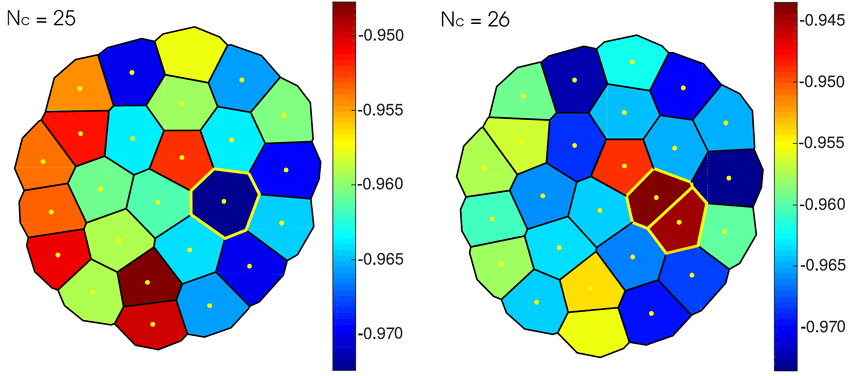
In the figure above, we can see two different partition sets: The first one denotes a Voronoi diagram with 25 partitions, while the second one has 26 partitions, where one cell splits into two cells (denoted with the red color). Typically, each cluster will encapsulate a set of data points; the critical aspect to consider in this method is to define the correct number of cells so as not to underfit or overfit the model (i.e. we don’t want a single cell for a single data point)
3.1.2 Hierarchical clustering
Hierarchical clustering methods are categorized into agglomerative and divisive. Agglomerative clustering involves isolating data points as separate groupings and merging them iteratively based on similarity until one cluster is achieved. There are four primary similarity measurement methods used in agglomerative clustering, which include:
- Ward’s linkage: A method similar to ANOVA in which the linkage function determining the distance between two clusters is calculated by computing the increase in the error sum of squares (ESS) after fusing two clusters into a single cluster.
- Average linkage: The linkage function is calculated by finding the average distance between objects in the first and second clusters.
- Complete (or maximum) linkage: This method involves starting with each element in its own cluster and then sequentially combining clusters until all elements are in the same cluster. It’s also referred to as “farthest neighbors clustering.”
- Dendrogram: The resulting clustering can be represented as a dendrogram, which displays the sequence of cluster fusion and the distance at which each fusion occurred.
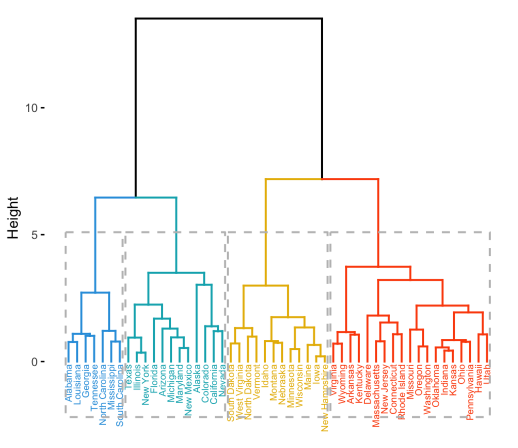
- Single (or minimum) linkage: This method combines two clusters in each step based on the closest pair of elements that don’t yet belong to the same cluster.
In divisive clustering, in contrast, a single data cluster is divided based on the differences between data points.
4. Active Learning
Active learning (AL), also known as optimal experimental design, allows for interactive labelling of data by the user with the desired outputs using an information source called a teacher or oracle.
This technique is useful when labelling data manually is costly, and there is an abundance of unlabeled data. As the learner chooses the examples, the number of examples required for learning a concept can be much lower than in normal supervised learning. In such scenarios, learning algorithms can actively seek labelling from the teacher.
As a reference, the Google Cloud project offers two pricing tiers per 1,000 units per human labeller; Tier 1 pricing applies to the first 50,000 units per month, and Tier 2 pricing applies to the next 950,000 units per month in the project, up to 1,000,000 units:
| Data type | Objective | Unit | Tier 1 | Tier 2 |
|---|---|---|---|---|
| Image | Classification | Image | $35 | $25 |
| Image | Bounding box | Bounding box | $63 | $49 |
| Image | Segmentation | Segment | $870 | $850 |
| Image | Rotated box | Bounding box | $86 | $60 |
| Image | Polygon/polyline | Polygon/Polyline | $257 | $180 |
| Video | Classification | 5sec video | $86 | $60 |
| Video | Object tracking | Bounding box | $86 | $60 |
| Video | Event | Event in 30sec video | $214 | $150 |
| Text | Classification | 50 words | $129 | $90 |
| Text | Entity extraction | Entity | $86 | $60 |
Based on the abovementioned costs, labelling 100,000 images with approximately five bounding boxes and two labellers per image for a specialized ML model would cost USD$112,000. Similarly, if we label 10,000 medical images, where each image requires about 15 semantically segmented objects and three labellers for accuracy, the cost would be roughly USD$391,500.
Labelling costs could be even higher for larger projects, which is the case for many current large-scale models. However, Active Learning can help reduce training costs significantly by predicting the missing labels, thus bypassing the need for extensive labelling. This technique, called inductive bias, involves reducing the version space for the problem by predicting missing labels.
In general, data points to be labelled are selected and prioritized strategically over less relevant data points. This approach often results in better outcomes than randomly selecting data points for labelling.
Crowdsourcing frameworks such as Amazon Mechanical Turk (MTurk) have implemented this method, allowing workers to label data provided by requesters and participate in the active learning loop of the model.
4.1 Process overview
The basic idea behind Active Learning algorithms can be summarized as follows:
Given a total sample of data  , the following steps are taken:
- A small subset
 of the data set is manually labelled.
 - The model is trained on the labelled subset .
- After training, the model is used to predict the class of the remaining data points.
- A score is assigned to each unlabeled data point based on the predictions made by the model.
- Based on the prioritization score, a strategy is chosen to select the next set of data points to be labelled.
- The process can be iteratively repeated by training a new model on the newly labelled data set, updating the prioritization scores, and selecting the next set of data points to be labelled until the desired level of accuracy is achieved.
There are three main sub-sampling strategies we can use in an Active Learning approach:
- Committee-based Strategies
- Large margin-based Strategies
- Posterior probability-based Strategies
4.2 Committee-based strategies
When multiple models are built, informative data samples can be selected from the predictions generated by these models. This ensemble of models is referred to as a committee. If the committee contains different models, a single data sample can have predictions. Sampling can be based on voting, variance produced (in the case of a regressor), or disagreement between the models.
There are three main approaches to committee-based strategies. We will only discuss the first method since it applies to various problems. The other two methods can be studied in more detail using the provided links:
- Query by Committee (QBC)
- Entropy-based Query by Bagging (EQB)
- Adaptive Maximum Disagreement (AMD)
4.2.1 Query-by-Committee (QBC)
This method was initially introduced by Seung et al. in 1992[1].
The approach employs disagreement among a group of hypotheses to choose data points for labelling. Two practical implementations of this approach are Query by Bagging and Query by Boosting, which use Bagging and Boosting to construct the committees.
The overall process can be summarized in the following steps:
- Construct a committee
 of models
  , where
  can be any real positive number greater than 1. A committee can also be referred to as an ensemble of models. To achieve this, we can use the following:
- Query by Bagging
- Query by Boosting
- The sum of committee models must represent some area of the version space.
- All models above are being trained on
 , where is our labeled set.
 - Whenever one query (unlabeled data point) comes in, our committee models will have competing hypotheses as to which label is the right one; each model will provide a vote.
- We will then devise a way to measure committee disagreements (i.e. how similar or different two probability distributions are). We can use the following:
- Vote entropy
- Kullback–Leibler divergence (KL divergence)
- Jensen–Shannon divergence (JS divergence), or information radius (IRad)
Vote entropy can be defined using the following expression:

Where:
 is a label.
 is the vote.
- is the committee size.
For a discrete random variable, the KL divergence can be expressed in terms of the logarithmic ratio of two PMFs:

Where:
 is the set of all possible variables for .
 is the probability mass function (PMF) of a given discrete distribution.
 is the probability mass function (PMF) of a given discrete distribution.
- Both and are defined on the sample space .
Which calculates the expectation of the logarithmic difference between the probabilities  and
and  , where the expectation is taken using the probability .
For a continuous random variable, we modify the KL divergence expression to include PDFs instead of PMFs:

Where:
 is the probability density function (PDF) of a given continuous distribution.
 is the probability density function (PDF) of a given continuous distribution.
Upon careful observation, we can see that the ratio used in both expressions allows us to compare two probability functions, whether they are probability mass functions (PMFs) or probability density functions (PDFs). For any input , the value of the ratio shows us how much more likely is to occur under compared to .
If the ratio value is larger than 1, is the more probable model. On the other hand, if the ratio value is smaller than 1, is the more probable model.
When the logarithm is taken, a  ratio value of 0 indicates that both models fit the data equally well. However, values larger than 0 suggest that
  is the better model, meaning it fits the data better. Conversely, values smaller than 0 indicate that
  is the superior model.
Finally, the JS divergence is based on the KL divergence; we have the following expression:

Where:


Upon careful examination, we can notice that the JS divergence approach has a similar treatment to the KL divergence approach. The primary distinction is that the JS divergence calculates the geometric mean of the differences between the two distributions.
4.3 Large margin-based strategies
A margin-based learning algorithm is an algorithm that chooses a hypothesis by minimizing a loss function  while using the margin of distances contained in the subset
  of labelled or training examples.
Below are the general steps involved in the process:
- The algorithm is given a set of training examples,
 , drawn from a specific distribution.
 - A version space
 is provided.
 - A margin function
 is defined, representing the margin of an example concerning the hypothesis function.
 - A margin-based loss function
 such as the one mentioned above is provided.
 - The margin-based algorithm
 returns a hypothesis scoring function
  that minimizes the loss over the training examples to choose a hypothesis scoring function.

There are some margin-based loss functions we can use, one being the hinge loss which is widely used in SVM models:

A margin-based active learning approach employs a margin function  in conjunction with a querying function
  by assuming that the current classifier typically makes accurate predictions on the training data. The algorithm selects those unlabeled examples with the smallest margin and, consequently, the lowest certainty.
There are two primary approaches to margin-based active learning. However, we will only elaborate on the first approach since it constitutes the generalized version. The second approach, Margin Sampling-closest Support Vectors (MS-cSV), can be studied in more detail using the following link:
- Margin Sampling (MS)
- Margin Sampling-closest Support Vectors (MS-cSV)
4.3.1 Margin Sampling (MS)
Margin Sampling (MS) is a method specific to the margin-based active learning approach that takes advantage of the geometric properties of Support Vector Machines (SVM).
For a binary classification problem with a labelled training set  and the corresponding labels
  , the primary objective of MS is to select examples with the smallest distance to the decision boundary from a set of
  unlabeled samples.
In a binary classification problem, the distance between a sample and the decision boundary can be expressed as:

Where:
-
 is a kernel matrix.
 -
 is the support vector coefficient.
 -
 is the support vector.
 -
 is the support vector candidate.
 - are the labels of the support vectors.
Therefore, the candidate selected into the training set is the one respecting the following condition:

After selecting the example  with the minimum distance to the decision boundary in the set of unlabeled samples, the algorithm adds and its true label to the labelled training set while simultaneously removing from the unlabeled training set
  .
.
4.3.2 Margin Sampling-closest Support Vectors (MS-cSV)
This strategy involves storing the positions and distances of each data sample from the support vectors. For each support vector, the algorithm selects a data sample that has the smallest distance from that support vector. As a result, we can have more than one unlabeled data sample in every iteration, eliminating the disadvantage of simple margin sampling, which only selects a single data sample for querying a human oracle per iteration.
4.4 Posterior probability-based strategies
A Bayesian Neural Network (BNN) is an extended classical Neural Network with posterior inference to control over-fitting. More generally, the Bayesian approach applied to a conventional Neural Network results in a probabilistic model; everything has a probability distribution attached to it, including model parameters (weights and biases in neural networks).
We can still take an input vector and feed it through a BNN, but the result will be a distribution instead of a single value. In other words, if we provide an input to the network, the BNN will assign a probability to each possible output.
Gaussian Processes (GPs) are probabilistic models as well. GPs relate to BNN in that a Neural Network with a single layer converges to a GP when its layer width is taken to infinity. Furthermore, in the case of a BNN, the weights are distributions, and the mean and covariance can be estimated by drawing samples from the weight distributions and calculating forward passes. For a non-Bayesian network, the Dropout can be used instead.
This relationship is interesting because it allows us to approximate a BNN to a Gaussian Process. This is relevant because Gaussian Processes are fully defined by their mean  and covariance
  functions. Thus we can compute the network’s mean and covariance for the unlabeled and labelled points.

The above diagram displays a plot of one-dimensional outputs of a neural network for two inputs against each other. The black dots represent the neural network’s computed function for these inputs with randomly drawn parameters from a distribution called  . The red lines represent the probability iso-contours for the joint distribution of network outputs induced by . Essentially, this distribution in function space corresponds to the distribution in parameter space, and the black dots are samples from this distribution. For neural networks that are infinitely wide, the distribution over functions computed by the NN is a Gaussian process. Thus, for any finite set of network inputs, the joint distribution over network outputs is a multivariate Gaussian.
Let us assume we have already trained a BNN on some labelled data and want to know which unlabeled points should be labelled to improve the model. We want to choose points for which the network has high uncertainty. When we add such points to the training data, the uncertainty will probably reduce, and the predictions will improve.
The estimated mean and covariance, using the approach above, completely define the Gaussian Process approximation of the Neural Network. The process defines the so-called posterior variance for every point in the pool. This variance is precisely the measure of uncertainty needed for Active Learning: If a point in the collection has a high variance, the network has a high uncertainty about its prediction, and the point should be selected.
After adding several high variance points from the unlabeled subset to the labelled subset, the network training is resumed, and the model quality should improve. This switch between adding points and re-training the network is usually performed iteratively until we get the accuracy we’re looking for.
5. Transfer Learning
Transfer Learning (TL) is an ML methodology that focuses on storing knowledge gained while solving one problem and applying it to a different but related problem. Transfer Learning is mainly used in Deep Learning given the massive resources required to train DNNs or the large and challenging datasets on which deep learning models are trained.
5.1 Process overview
Before we dive into specifics, let us generalize and consider a source Deep Neural Network we would like to train and transfer to another problem.
In a general way, a TL approach consists of the following steps:
- Train the source DNN on a base dataset, or get a pre-trained model.
- Create a new base model replacing the last layer from the source model.
- Freeze layers.
- Add new layers and train them on our new data set.
- Improve the model via fine-tuning.
Let us explain in detail each of the steps involved:
5.1.1 Training the Source DNN
This step is critical since the transfer success will heavily depend on the source model we select. We can either build a source model and train it ourselves or select a pre-trained model. The main thing to remember is we need to ensure that we have a strong correlation between the knowledge of the source model and the target domain for them to be compatible.
For pre-trained models, specifically DNNs, we have some options:
- Computer Vision
- VGG-16
- VGG-19
- Inception V3
- XCeption
- ResNet-50
- NLP
- GPT-3
- Microsoft MT-DNN
- Google BERT
- RoBERTa
- Huggingface Transformers
- ULMFit
- XLNet
- Word2Vec
- GloVe
- FastText
5.1.2 Establishing a Base Model
Our base model architecture must closely resemble the source model we choose to employ. We have two options: either we can download the pre-existing network weights, which will save us the time of further training, or we will have to train our model from scratch using the network architecture.
5.1.3 Freezing Layers
Freezing layers selectively is a crucial step in Transfer Learning. This entails freezing the initial layers from the pre-trained model to evade the additional work of teaching the basic model features.
If we fail to freeze the initial layers, we will lose all the learning that has already transpired. This will be no different from training the model from scratch and will waste time and resources.
5.1.4 Adding and Training New Layers
The frozen layers must consist exclusively of the generalized aspects of our dataset. If we freeze too many layers, our model will be incapable of generalizing to the task at hand; conversely, if we remove too many layers, it will exert the extra effort of learning what it already knows.
As a result, the new layers should be used to predict the specialized tasks of the model, typically comprising the final output layers.
Once we have the added layers, we must train them using our target dataset; the pre-trained model’s final output is likely to differ from the output we require for our model. For example, pre-trained models trained on a given dataset may output a different number of classes than we require for our specific target model.
Thus, we must train the last layers with our dataset to ensure that the output meets our problem’s specifications.
5.1.5 Refining the Transferred model
To improve the accuracy of the transferred model, we may need to fine-tune the frozen layers, depending on the accuracy of the source model we chose and how similar the source dataset is to our target dataset.
Fine-tuning consists of unfreezing some parts of the base model and training the entire model again on the whole dataset with a shallow learning rate. This technique can help increase the model’s performance on the new dataset while preventing overfitting.
It may be necessary to repeat this step multiple times until we achieve a transferred model that meets the requirements of our problem.
5.2 Transfer Learning strategies
Depending on the problem we’re trying to solve, the domain of the application, and the availability of datasets, there are three main strategies for TL:
- Inductive Transfer Learning
- Transductive Transfer Learning
- Unsupervised Transfer Learning
The selection of an appropriate transfer learning strategy depends on various factors, including the problem to be solved, the application’s domain, and the datasets’ availability.
Generally, there are three primary strategies for transfer learning, and they can be determined by answering three key questions:
- What aspects of knowledge can be transferred from the source domain to the target domain to improve the target task’s performance?
- When should knowledge transfer be utilized, and when should it be avoided, to ensure improved performance in the target task without degradation?
- Given the specifics of the target domain and task, how should knowledge be transferred from the source model to the target model?
Answering these questions helps determine which transfer learning strategy to use for a particular task.
5.2.1 Inductive Transfer Learning
In this scenario, the source and target domains are the same, yet the source and target tasks differ. The algorithms utilize the source domain’s inductive biases to help improve the target task. Depending upon whether the source domain contains labelled data or not, this can be further divided into two subcategories, similar to multitask learning and self-taught learning, respectively.
5.2.2 Transductive Transfer Learning
In this scenario, there are similarities between the source and target tasks, but the corresponding domains are different. In this setting, the source domain has a lot of labelled data, while the target domain has none.
5.2.3 Unsupervised Transfer Learning
This setting is similar to inductive transfer, focusing on unsupervised tasks in the target domain. The source and target domains are similar, but the tasks are different. In this scenario, labelled data is unavailable in either of the domains.
Transfer Learning is an extensive and ever-growing topic, and there’s a wide range of techniques specific to given domains. We will not cover further details on this segment. Still, an in-depth review containing additional strategies and mathematical modelling can be found here.
6. Reinforcement Learning
Reinforcement Learning (RL) is an ML technique that enables a model to learn in an interactive environment by trial and error using feedback from its own actions and experiences; in short, the model will learn from its own mistakes using a system of rewards and punishments as signals for positive and negative behaviour.
Compared to unsupervised learning, reinforcement learning is different regarding goals. While the goal in unsupervised learning is to find similarities and differences between data points, in the case of reinforcement learning, the goal is to find a suitable model that would maximize the total cumulative reward of the agent.
Some key terms that describe the basic elements of an RL problem are:
- Environment: Physical world in which the agent operates.
- State: Current situation of the agent.
- Reward: Feedback from the environment.
- Policy: Method to map agent’s state to actions.
- Value: Future reward an agent would receive by acting in a particular state.
A generalized RL algorithm follows the step-by-step process below:
- Initially, the RL agent observes the current state of the environment.
- The agent selects an action to take based on the current state.
- The environment responds with a new state and a reward signal.
- The agent receives the reward signal and updates its knowledge of the environment and the value of the action taken.
- The agent then utilizes the updated knowledge to choose the following action.
- This process repeats iteratively, with the agent learning from the feedback received at each step and adjusting its behaviour accordingly.
- Eventually, the agent’s actions will converge towards an optimal policy that maximizes the expected long-term reward.
This process can be represented as a feedback loop, where the agent interacts with the environment and receives feedback in the form of rewards. The agent’s ultimate goal is to learn the most suitable sequence of actions to maximize the cumulative reward over time.
RL algorithms can be categorized as model-based and model-free methods and value-based and policy-based methods, depending on the approach used to learn and optimize the policy.
The model-based and model-free classification types can be summarized as follows:
- Model-Based RL: Learn a model of the environment, which can be used to simulate future states and rewards. This allows the agent to plan ahead and make informed decisions.
- Model-Free RL: Do not learn a model of the environment. Instead, they directly learn a mapping from states to actions and use trial and error to improve this mapping over time.
- Hybrid RL: Combine elements of both model-based and model-free approaches, allowing for more flexible and efficient learning.
The value-based and policy-based classification types can be summarized as follows:
- Value-Based RL: They learn by estimating the value of each state or state-action pair in the environment. These algorithms aim to find the optimal policy that maximizes the expected cumulative reward by learning the optimal value function.
- Policy-Based RL: They learn by directly searching for the optimal policy, which is a mapping from states to actions that maximize the expected cumulative reward. These algorithms learn a parametric or non-parametric representation of the policy that can be optimized using gradient-based methods.
There are several types of RL algorithms available. Below are some of the most common ones:
- Q-Learning
- State-Action-Reward-State-Action (SARSA)
- Actor-Critic
- Deep Reinforcement Learning (DRL)
- Policy Gradients
- Monte Carlo Methods
- Temporal Difference (TD) Learning
RL algorithms present several advantages, including:
- Flexibility: RL can be applied to various applications, from games to robotics to financing. It can learn to perform complex tasks that would be difficult or impossible to program directly.
- Adaptability: RL algorithms can adapt to changes in the environment, making them useful in dynamic and unpredictable settings.
- Efficiency: RL algorithms can learn quickly from large amounts of data, making them useful in applications where speed is crucial.
- Generalization: RL algorithms can generalize what they have learned to new situations, allowing them to perform well in problems they have not encountered before.
- Optimization: RL algorithms can optimize complex and non-linear systems, finding the best policies to achieve a particular goal.
Classification by Parametric and Non-Parametric models
As we have seen, machine learning models can be classified by the types of inputs they accept as well as their functioning. We can also look at ML algorithms regarding how they map data points.
1. Parametric Models
Parametric models are machine learning models that use a mathematical equation to relate inputs and outputs. For example, Linear Regression is a parametric model that uses a straight-line equation to fit data points on a plane, while Logistic Regression uses the sigmoid function to classify data. These models are based on predetermined mathematical formulas to generate outputs.
Other examples of parametric models include:
- Perceptrons
- Simple Neural Networks
- Linear Support Vector Machines
Parameters of these models can include:
- The coefficients of the equation of a straight line in Linear Regression.
- The coefficients of a polynomial in Non-linear Regression.
- The support vectors in a Support Vector Machine.
- The weights in a Neural Network.
2. Non-parametric models
In contrast, Non-parametric models do not make strong assumptions about the form of the mapping function; they instead learn from the data itself. A prevalent supervised example would be the Decision Tree Classifier, which is based on a hierarchical structure.
Other non-parametric examples include:
- k-Nearest Neighbors (KNN)
- Random Forests
- Gradient Boosting Machines (GBM)
- Support Vector Machines with non-linear kernels (SVM)
- Neural Networks (NN)
- Gaussian Mixture Models (GMM)
- Principal Component Analysis (PCA)
3. Parametric vs Non-parametric models
This question is trickier since it implicates the nature of the problem we’re trying to solve. Still, we can summarize both models in a comparative table to have a better understanding of the two types:
| Parameter | Parametric Models | Non-Parametric Models |
|---|---|---|
| Parameter usage | Use a fixed number of parameters to build the model | Use a flexible number of parameters to build the model |
| Data assumptions | Consider strong assumptions about the data | Consider fewer assumptions about the data |
| Computational effort | Are usually less computationally expensive | Are usually more computationally expensive |
| Performance | Are usually faster performing due to a predefined set of parameters | Are usually slower due to undefined parameters |
| Data volume requirement | Usually require less data | Usually require more data |
| Simplicity | Are usually simpler and easier to understand | Are usually more complex since we don’t fully know the underlying model |
| Flexibility | Are less flexible since they assume one fixed functional form | Are extremely flexible since there’s no predefined functional form |
| Accuracy | Can, in some cases, be less accurate if the data is complex or does not fit the underlying model | Can be highly accurate if the data is complex, but can also cause overfitting |
Classification by Generative and Discriminative models
Another way to classify ML models is to think of them in terms of how they model a solution to the problem we’re trying to solve; we can divide them into two main types:
- Generative models
- Discriminative models
Both methods can be used for classification purposes and categorized as supervised, semi-supervised or unsupervised.
1. Generative models
Generative models aim to populate datasets by modelling their joint probability distribution,  . They predict conditional distributions to populate a specific class with data points. These models rely predominantly on probability distributions to populate classes.
The training process of a generative model involves learning the parameters of the probability distribution. There are many types of generative models, but they all share the same basic idea of learning a probability distribution that can generate new data.
Once the model has been trained, it can be used to generate new data by sampling from the learned distribution. The process of generating new data can be done in various ways depending on the specific type of generative model.
For example, a Gaussian mixture model (GMM) can generate new data by sampling from a mixture of Gaussian distributions. Similarly, a generative adversarial network (GAN) generates new data by pitting two neural networks against each other: one network generates new data, while the other tries to distinguish between the generated data and real data from the training set.
To better illustrate the concept, let us consider a classification example:
- We are presented with a labelled dataset consisting of two labels:
 .
. - Our objective is to train a model to accurately classify new data points as either
 or
or  .
. - A Generative model creates two separate models, one describing the distribution of points and another describing the distribution of points. It learns the distribution of each class, which is a function that describes the likelihood of observing a particular feature vector given the class label. The models can be thought of as probability density functions that describe the data distribution for each class.
- When presented with an unseen data point, our model determines probabilistically to which distribution it is most likely to belong.
Thus, the decision boundary for a Generative model is determined by the probability or likelihood that a specific data point belongs to a given distribution.
Binary classification is one of the simpler generalizations, but Generative models can perform much more complex tasks, particularly in the painting and synthetic visual art generation:

Let us explain the generalized steps of how this is achieved:
- Collect a dataset of visual art: The first step in creating a generative model for visual art is to collect a dataset of visual art we want to generate new examples of. This dataset can include paintings, drawings, or any other type of visual art.
- Preprocess the dataset: Before training the generative model, we need to preprocess the dataset. This may include resizing the images, normalizing pixel values, and performing data augmentation to increase the size of the dataset.
- Train the generative model: The next step is to train the generative model using the preprocessed dataset. Several types of generative models can be used for visual art creation, such as Variational Autoencoders (VAEs), Generative Adversarial Networks (GANs), and Autoregressive models. During training, the generative model learns to generate new images similar to the images in the training dataset. The model is trained on a loss function that measures the difference between the generated and real images in the dataset.
- Generate new art: Once the generative model is trained, we can use it to generate new art. To generate a new piece of art, we sample a random noise vector from a normal distribution and pass it through the generative model. The model’s output is a new image generated from the learned distribution.
- Evaluate the generated art: The final step is to evaluate the generated art. This can be done using various metrics, such as perceptual similarity, diversity, and visual quality. The evaluation can improve the generative model by fine-tuning the model’s parameters or adjusting the loss function.
Now, let us explain in more detail how these models work:
- Variational Autoencoders (VAEs): They work by learning to encode an image into a low-dimensional latent space and then decode the latent vector back into an image. The model is trained to minimize the difference between the input and reconstructed images in the pixel space while encouraging the latent space to follow a normal distribution. Once trained, we can sample random points from the latent space and decode them into new images.
- Generative Adversarial Networks (GANs): They consist of two neural networks: a generator and discriminator networks. The generator is trained to generate images that fool the discriminator, while the discriminator is trained to distinguish between real and fake images. The generator network takes random noise as input and produces an image, while the discriminator network takes an image as input and predicts whether the image is real or fake.
- Autoregressive models: They model the conditional probability of each pixel in an image given the previous pixels. The model generates an image one pixel at a time, sampling from the conditional distribution for each pixel. The model is trained to maximize the log-likelihood of the training images.
Other generative models include:
- Gaussian Mixture Model (GMM)
- Naïve Bayes Classifier
- Hidden Markov Model (HMM)
- Boltzmann Machines
- Restricted Boltzmann Machines (RBMs)
- Deep Belief Networks (DBNs)
- Conditional Random Fields (CRFs)
2. Discriminative models
In contrast to Generative models, Discriminative models work by defining boundaries between classes. They learn to predict the labels of new examples based on their input features; the models are trained to minimize the difference between the predicted labels and the true labels in the training data.
Let us continue with the previous generalized binary classification example:
- Given that we have the same data set and want to classify new data points as or , a Discriminative model will build a boundary separating the two classes.
- It will not focus on analyzing the whole population; instead, it will look at the distance to the nearest data points and draw a boundary that separates them in the most optimal way.
We have already mentioned some examples of discriminative models in the previous classification types:
- Decision Trees (DT)
- Random Forests (RF)
- Gradient Boosting Machines (GBM)
- Support Vector Machines (SVMs)
- Neural Networks (NN)
- K-Nearest Neighbors (KNN)
- Linear Discriminant Analysis (LDA)
- Quadratic Discriminant Analysis (QDA)
- Maximum Entropy (MaxEnt)
3. Generative vs Discriminative models
It heavily depends on the problem we’re trying to solve and the nature and volume of our data set:
- In a classification problem context, a Generative model will generally underperform a Discriminative model in terms of execution time if we have a large data set. This is because the first considers the entire population, while the latter can ignore the points further from the decision boundary.
- Conversely, if we have a limited data set, a Discriminative model will generally underperform a Generative model in test accuracy since the latter will place a given structure on the model that will often prevent overfitting.
- If we are presented with unlabeled data, a Discriminative model will generally underperform a Generative model since the first doesn’t require labelled data; it learns by modelling distributions.
- If we would like to generate samples based on the assigned classes, a Generative model would offer the actual class distribution, from where we could easily sample data points. A Discriminative model would not provide such a distribution, thus, we could not generate samples.
We can summarize both models in a comparative table to have a better understanding of the two types:
| Parameter | Generative Models | Discriminative Models |
|---|---|---|
| Modeling | Learn the boundary between classes by building a probability distribution for each class. | Learn the boundary between classes providing classification splits |
| Assumptions | An underlying distribution | No underlying distribution |
| Complex relationships | Better at complex models | Underperforms in more complex models since it does not take the whole population into account |
| Probabilistic | Mostly probabilistic | Probabilistic or non-probabilistic |
| Training sample size | Require less training examples | Require more training examples |
| Overfitting | Prevent overfitting with limited data set sizes because of the generalized structure (distribution) of the classes | Are more prone to overfitting with limited data set sizes |
| Decision boundary | Traced where one model becomes more likely | Traced where the separation between classes is more optimal based on nearest data points |
| Labeled / Unlabeled data | Especially high-performing on unlabeled data | Not designed for unlabeled data |
| Computational performance | Decreases with increasing data set volume | Decreases less than with Generative models |
| Outlier detection performance | Generally work for outlier detection | Do not work well for outlier detection |
| Synthetic data generation | Can easily be used to generate data points from the modelled distributions | Cannot generate synthetic data since they do not consider a distribution (they do not have the full class picture) |
Next steps
There are multiple ways of approaching how to further learn about ML techniques depending on what we’re trying to achieve. In this article, we will mention three:
- An academic approach
- An engineering approach
- A consulting approach
Disclaimer: None of the links provided are affiliate links. The selected resources are of my own choosing.
1. An academic approach
Research Science / Machine Learning Science is mainly interested in developing new models using what we already have as theoretical basis and further expanding it. This approach is scientific in nature and involves rigorous and extensive experimentation applying domain knowledge from the following areas:
- Linear Algebra
- Differential and Integral Calculus
- Graph Theory
- Linear Programming
- Nonlinear Programming
- Convex Optimization
- Simulation Techniques
- Probability Theory
- Statistical Modeling
- Computer Science
Suggested material includes the following programs:
- Machine Learning with Python, MIT
- Supervised Machine Learning, Andrew Ng & Stanford
- Deep Learning Specialization, Andrew Ng
- Machine Learning with Python, IBM
- Machine Learning Specialization, Andrew Ng & Stanford
2. An engineering approach
Machine Learning Engineering is a discipline mainly interested in deploying developed and trained ML models in a production environment. This approach is more Software Engineering-oriented and involves domain knowledge from the following areas:
- Computer Science
- Full-Stack Software Engineering
- Parallel Computing
- ETL Techniques
- Cloud Computing
- Containerization & Orchestration
- DevOps & Agile Systems
Suggested material includes the following programs:
- CS50’s Introduction to Computer Science, Harvard
- Introduction to Machine Learning in Production, Andrew Ng
- MLOps Specialization, Andrew Ng
- Machine Learning Specialization, DeepLearning
- Machine Learning in Production, DataBricks
3. A consulting approach
Many companies in different sectors are in the look for new methods which allow them to optimize existing processes. Several firms specialize in providing Machine Learning Consulting services to clients to cover this demand. This approach is more Business-oriented and involves domain knowledge from the following areas:
- Business Consulting
- Project Management
- Software Engineering
- Cloud Computing
Suggested material would include the following programs:
4. Free learning resources
Finally, there are several YouTube channels providing high-quality content:
- sentdex
- Data School
- Artificial Intelligence – All in One
- DeepLearningAI
- Machine Learning with Phil
- Jeremy Howard
- StatQuest with Josh Starmer
- Stanford Online
- MIT OpenCourseWare
- freeCodeCamp.org
Conclusions
In this segment we discussed in a general way how a typical Machine Learning model is implemented and how it works. We mentioned 3 different types for classifying ML models according to how they learn, how they represent data associations and how they conceptualize a potential solution. We also discussed the most important subclassifications, the most relevant strategies currently available, the main models comprising them, and a simplified mathematical model for the most relevant cases. Finally, we performed some comparisons between subclasses and strategies, and gave an overall recommendation for when to use which one.
Machine Learning is getting all the attention since major breakthroughs have been achieved recently. With the exponential growth of data & processing power, and the increasing demand for intelligent systems, ML has become a critical component in many industries, from healthcare to finance, manufacturing to transportation.
Because so much can be done using ML, it’s important to know all the angles we can take in order to solve problems of different domains using ML techniques, while at the same time evaluating if this approach is the right one for our specific case.
This segment went over the tip of what can be done; there is extensive research currently being made on new methods and more sophisticated algorithms, and we’re just getting started.
References
- [1]Advances in Neural Information Processing Systems 5 (NIPS 1992)
- IBM, What is supervised learning?
- IBM, What is unsupervised learning?
- Machine Learning Mastery, What Is Semi-Supervised Learning?
- Towards Data Science, Active Learning in Machine Learning
- Analytics Vidhya, Commonly used Machine Learning Algorithms
- Research Gate, Spam-detection Features
- KD Nuggets, Managing Unbalanced Data
- DataRobot, Semi-supervised Learning
- IBM, Unsupervised Learning
- Laura E. Wadkin, Sirio Orozco-Fuentes, Irina Neganova, The recent advances in the mathematical modelling of human pluripotent stem cells
- Neptune AI, Active Learning Strategies
- Abbassi Saber Nawfal, Active Learning Scenarios and Techniques
- Anna-Lena Popkes, Kullback-Leibler Divergence
- Maria-Florina Balcan, Andrei Broder, and Tong Zhang, Margin based Active Learning
- Dan Roth and Kevin Small, Margin-based Active Learning for Structured Output Spaces
- Machine Learning Mastery, Transfer Learning
- V7 Labs, A Newbie-Friendly Guide to Transfer Learning